Automobile Ride Quality Study
Introduction:
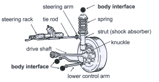
The purpose of this simulation is to model an automotive suspension and the effect it has on overall vehicle ride quality and comfort. Suspension systems must compromise between ride quality and vehicle handling, depending on the goals of the vehicle being designed. Sports cars have suspension systems that are designed for better handling by improving control of vehicle and reaction times; however, this affects the ride quality. On a sports car, the lower center of gravity is better for handling. However, the low ground clearance also limits suspension travel, requiring stiffer springs reducing ride comfort. Whereas a luxury vehicle will handle worse than a sports car but will provide a much more comfortable ride. If the suspension system is too soft, it can cause the passengers to develop motion sickness. On the other hand, if a suspension system is too harsh, the passengers will be subject to significant acceleration levels, which can lead to chronic medical conditions. See figure 1: automotive suspension system below.
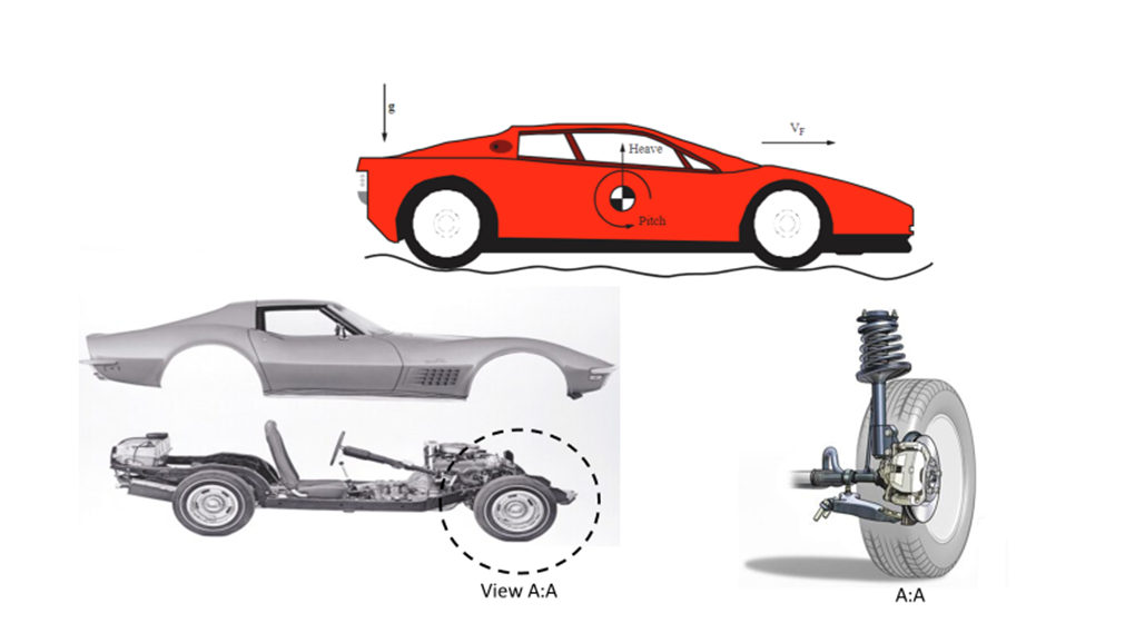
As ride quality improves inside of a vehicle, the comfort for the vehicle improves, providing a better experience for the passages. A good suspension system should avoid damaging any cargo inside the vehicle and should also help reduce driver fatigue on long trips while improving stability and maneuverability characteristics. Based on a study conducted by the International Standards Organization (ISO) humans are most sensitive to accelerations in the vertical direction. As a result, a good suspension system should absorb any disturbance on the road surface, such as potholes or debris, which can cause a driver to experience vertical velocities, thus reducing ride quality. In a worst-case scenario, a large disturbance can affect the driver’s ability to control the vehicle, putting anyone inside the vehicle in danger. See figure 2: Suspension system disturbance below.
Analysis:
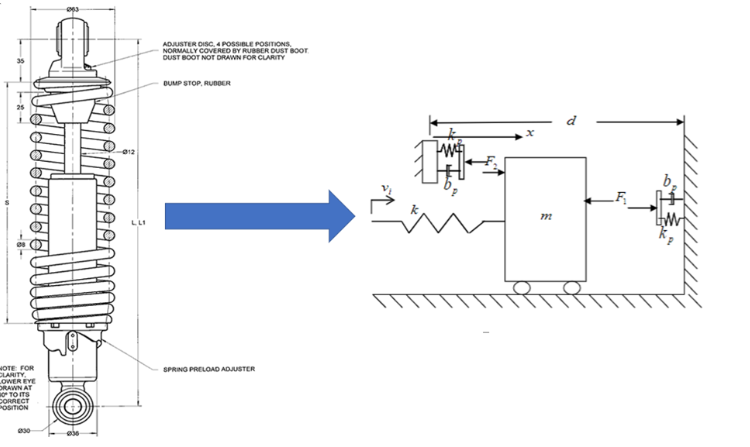
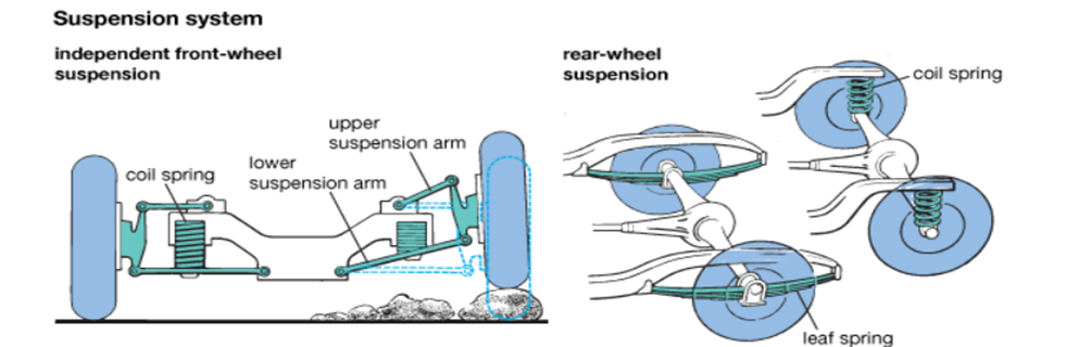
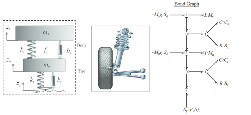
To simplify the analysis, the model only focused on understanding the affects to heave or vertical acceleration felt by the driver. For this project, any pitch or roll movement of the vehicle will be out of scope. Due to this simplification, the modeling will focus on just one corner of the vehicle. If the front of the vehicle moves up, the rear of the vehicle is assumed to also move up the proportional distance. The suspension system was modeled as having two main energy storage elements (mass) a sprung mass which is the mass of the vehicle being supported by the suspension system, and the un-sprung mass, which includes the wheel/tire and axle. Both mass elements are subject to the gravitational force which is opposing any vertical acceleration. The suspension system components are modeled as a spring (capacitor element) and a shock (resistor element) in parallel, which are connected to the un-sprung mass. Similar to the suspension system, the tire was also modeled as a spring and a damper in parallel. The tire transfers the road force to the un-sprung mass (wheel hub). See figure 3: Suspension model and bond graph below.
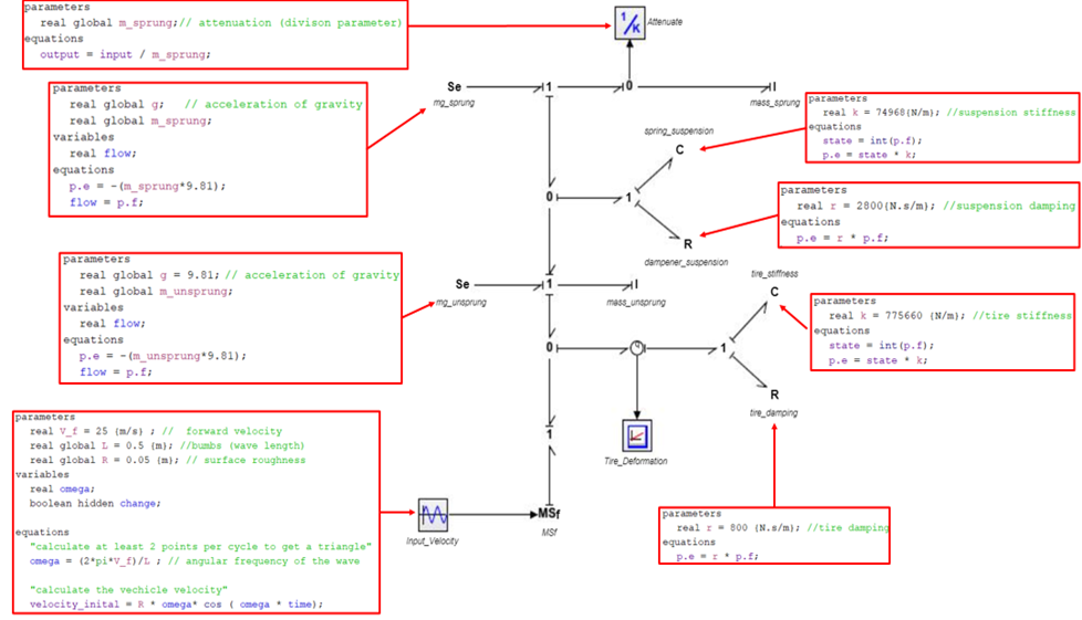
The final bond graph with code can be seen below in figure 4: bond graph model with code. This bond graph model is used to solve the first three problems since the input velocity is the same. To view file, see appendix section below.
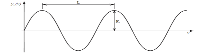
For the first three parts of this project; the only input to the system is the road profile that is modeled as a having sinusoidal curve bumps of wavelength (L) and the amplitude being the road roughness (R). The road profile, which is equal to the displacement of the tires (m) can be described with the following equation:

By differentiating the road profile with respect to time the following velocity (m/s) source is derived:
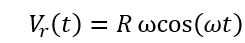
Where the frequency ω (rad/s) is equal to:

For this project it was assumed that the tires will have constant contact with the surface of the road. As a result, the road roughness can be considered a displacement or velocity source to the bond graph model. See figure 4: Road roughness at the top of the following page.
Results:
Part 1. Initial Response
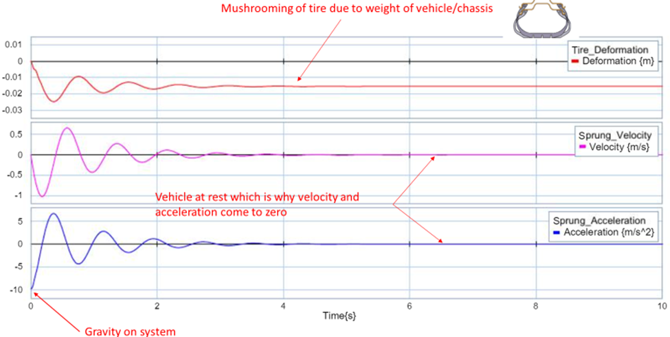
During the first part of this project you assume that your vehicle is at rest on a perfectly flat road with zero initial tire deflection. As a result, at the begin of the simulation the only force acting on the system is the force of gravity on both the sprung and un-sprung mass, which is why the initial acceleration on the system is -9.8m/s2. However, the acceleration peaks at the max deflection of the tire (~-.025mm) and quickly decays afterwards, as the systems achieves a stead state. The max velocity seen is -1m/s, which is seen at the beginning of the system, prior to the tire achieving its max deflection, as the gravitational energy exerted on the mass is converted into kinetic energy. Once the system comes to achieves equilibrium ~4seconds into the simulation, you can find the static deflection of the tire at -0.015m. See figure 6: Initial Response plots below.
Part 2. Frequency Dependence
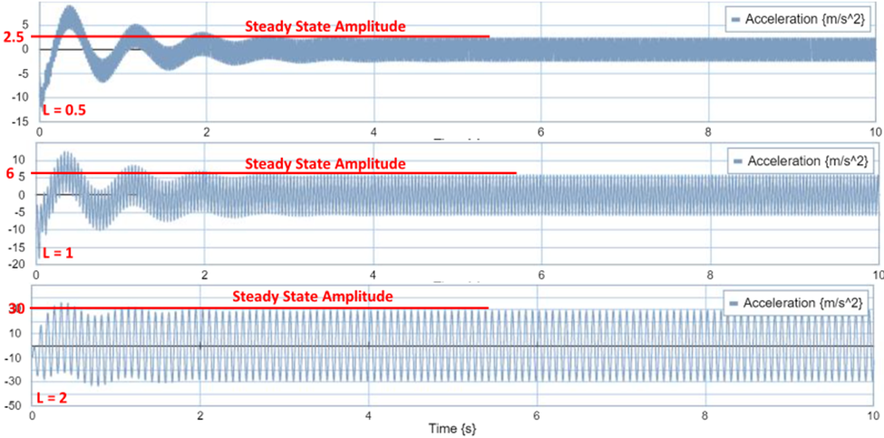
During the second part of this simulation we had to find the frequency response plot using both a numerical integration and frequency response approach on 20sims. For the numerical integration response, the wavelength L was varied from 0.5 to 50m, and a total of 12 runs were simulated to determine the amplitude of the steady state sprung mass acceleration. See figure 7: steady state amplitude which is an example of the first 3 trials conducted L =0.5, L =1, L =2.
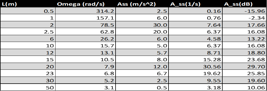
To convert the steady state acceleration to normalized stead state acceleration, take the steady state acceleration found after running each model and divide it by road roughness (0.05m) and ω (rad/s). To convert the normalized steady state acceleration to the correct units (dB) take 20*log10 of your previous answer. The whole data set can be seen below in table 1: normalized steady state acceleration.
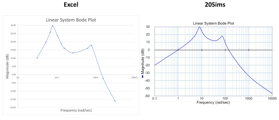
Finally, the frequency (ω) was plotted against the normalized steady state acceleration. This same plot was constructed using the frequency response approach on 20sims. The result from these two graphs are identical, the 20-sim model is more complete since the excel only used 12 data point to plot the graph. Both graphs show that the system has two worst bump frequencies, the first is when ω = 7.9 rad/s and the second one is when ω = 78 rad/s. The magnitude of these frequencies is 30dB and 18dB respectively. See figure 7: Bode frequency dependence plot below.
The greater the magnitude (dB) the worse the ride quality is of the vehicle. Since the vertical acceleration of the vehicle is assumed to be a constant 25m/s the only variable really effecting the frequency are the bumps (wavelength) L. As a result, it can be assumed that if the road profile consists of many small bumps (ω < 1) the ride quality of the vehicle will be good. The reason behind this is because the variation in the road is so small that the tire just rolls any disturbance on the road. However, as the size of the bumps begin to increase (1<ω < 100), the tire is no longer able to absorb all the variation on the road. This causes the tires to move up and down very rapidly leading to very poor ride quality for the passengers. Finally, when the road profile consists of very long bumps (ω > 100) even though the tires is going up and down the amplitude of each bump is so spread out that the variation is barely noticeable, leading to very good ride quality. See figure 8: Tires and road profile.

Part 3. Parameter Variation
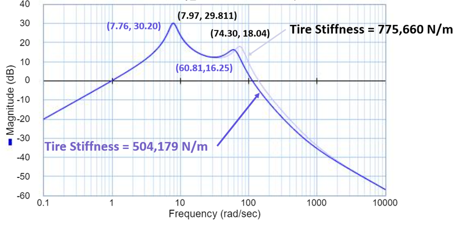
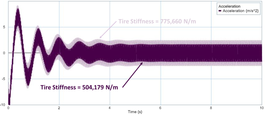
In the third part, the goal was to understand the effect of tire stiffness and sprung mass on overall ride quality. For the first part, the tire was assumed to be deflated, causing the tire stiffness to decrease by 35% from 775,660 N/m to 504,179 N/m. The result of deflating the tire pressure was an improvement in overall ride quality after a frequency of 30 rad/sec. It was a small shift, but the magnitude of the second worst bump decreased from 18 dB to 16dB. The reason behind this was since the tire was not as stiff on the second run, it could deform more, resulting in an improved ride quality. When comparing the effect of deflating the tire has on the sprung mass, during the transient response (0-4 seconds), the difference between both graphs was minor. However, the vertical acceleration of the non-deflated tire was always greater. As the vertical velocity settles down and approaches a steady state response, the difference in vertical acieration is much more noticeable. The vertical acceleration experienced by the driver for the non-deflated tire was about 2.5m/s2, while the acceleration experienced by the driver for the deflated tire was about 1 m/s2. See figure 9: Deflated tire – bode and acceleration graph below.
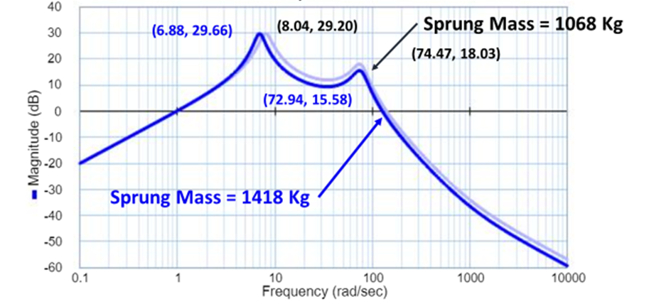
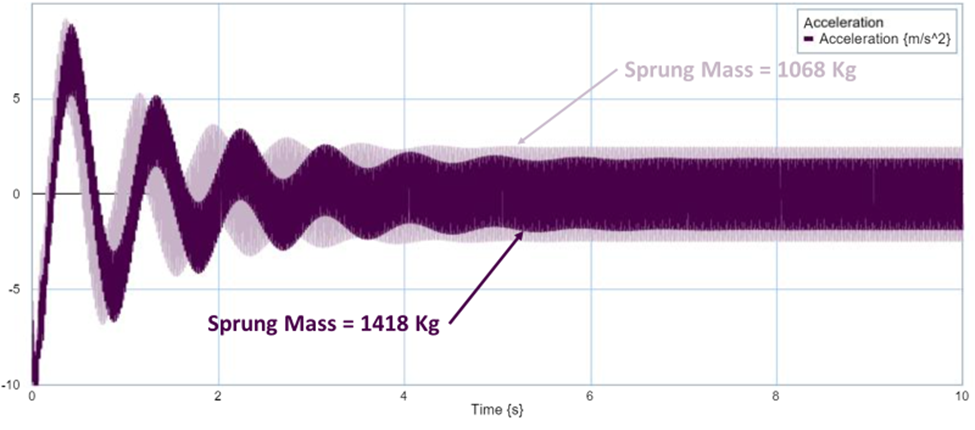
During the second part of this simulation, it was assumed that 5 passengers were picked up, each averaging 70kg each, adding 350kg to the sprung mass. The result of the additional sprung mass added to the vehicle was a slight shift to the left of the first worst bump frequency. Even though the magnitude of the first bump frequency was the same, the heavier vehicle hit the worst bump frequency at 6.88 rad/sec while the original vehicle achieved the same worst bump frequency at 8.04 rad/sec. After the first worst bump frequency, the heavier vehicle also experienced a quicker decay than the original vehicle. The magnitude of the second worst bump was also lower at only 15.58dB compared to 18.03dB. The lower magnitude seen in the bode plot of the heavier vehicle means that the overall ride quality has improved. When comparing the acceleration graph for both scenarios, both graphs start the same because of gravity. However, the heavier vehicle quickly gets out of phase from the original vehicle during the transient response. Even though the vertical acceleration is comparable in both scenarios, the heavier vehicle is taking longer to achieve the same vertical acceleration. During the steady state response, the vertical acceleration for the heavier vehicle is lower at only 1 m/s2 versus the original vehicle, which has a vertical acceleration of 2 m/s2. See figure 10: Increased mass – bode and acceleration graph below.
Discussion:
Since the force applied to the system was a harmonic force (Vr(t)) all the graphs have a similar shape. At the beginning, each the graph is largely influenced by the transient response, which is why we notice so much fluctuation for the first few seconds of all the graphs. However, this will converge to the steady state response after some time. Overall, the quicker the graph achieves steady state and the lower the magnitude of the vertical acceleration, the better the overall ride quality of the vehicle. When reviewing the bode plots the lower the magnitude of the graph and the quicker the graph decays over time, the better the overall ride quality of the vehicle.
Conclusions:
When designing a vehicle, an automaker must make sure that the vehicle being designed is balanced and is making the right decision is being made based on the target consumer. Even though each automaker will try to optimize their suspension system by calibrating their vehicle suspension (spring and shocks). There will come a point where you can only improve the performance of your suspension system so much and to improve the performance even further will require additional capital. Depending on the vehicle and the program’s budget, this might or might not be the correct move. However, there are factors which improve the overall vehicle ride quality, but they are directionally incorrect for the vehicle. Decreasing the recommend tire pressure of the vehicle might improve ride quality, but it will also increase rolling resistance of the tire, causing for increase fuel consumption or decrease vehicle range. Increase the overall vehicle mass is another factor which might improve ride quality but will reduce vehicle max speeds and acceleration times. In addition, adding more mass to the vehicle will also decrease the vehicles efficiency, reducing fuel economy and range. Automakers sell vehicle, not suspension systems, and as a result need to make sure the vehicle is optimized based on intended hardware, but well-balanced between all the different vehicle systems and is not to basis to any one system.