The Role of Resonance in RL and RC Circuit: How to Design and Analyze Circuits with Resonance

Hey everyone! Today, we’re diving into the fascinating world of RCL circuits and uncovering the magical phenomenon called “resonance.” If you’re into electronics and circuits, this is going to blow your mind!

What Are RCL Circuits?

So, first things first, let’s get to know what RL and RC circuits are all about. These simple circuits containing dc sources, resistances, and one energy storage element:

1. Capacitor (RC): Picture this as a little storage unit for electrical charge. It accumulates energy when the voltage across it changes, and it can release that energy later on.
2. Inductor (RL): When current flows through it, it creates a magnetic field. If the current changes, the magnetic field changes too, and this induces a voltage in the inductor.

What is the difference between first-order and second-order RLC circuit?

The main difference between first order and second order RLC circuits lies in their complexity. First-order RLC circuits contain only one energy storage element (RL and RC circuits), while second-order RLC circuits have two (both a capacitor and an inductor), leading to more intricate behavior and responses to input signals.

The Exciting World of Resonance

Alright, now that we know what RC and RL circuits are made of, let’s get to the juicy part – resonance! Resonance happens when something in our circuit starts to vibrate or oscillate like crazy. Imagine pushing a swing and finding the perfect rhythm to make it go higher and higher with less effort – that’s resonance! Other examples of resonance are sympathetic vibrations of pendulums, machine parts, instruments, air column and tuning fork, oscillations of bridge.

Getting to Know Resonant Frequency

Resonance in RCL circuits occurs at a particular frequency, which we call the “resonant frequency. At this frequency, the reactance of the capacitor and inductor cancels out each other, leaving only the resistance to limit the current.

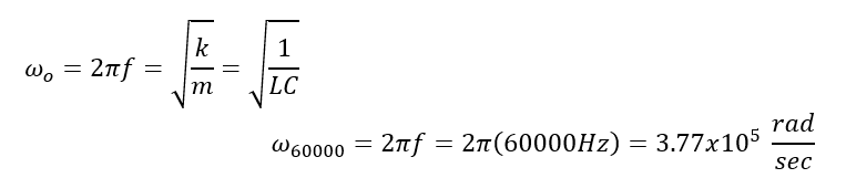
The formula to calculate the resonant frequency (f) is straightforward:

f = 1 / (2 * π * √(L * C))

Where:

• f is the resonant frequency in Hertz (Hz).
• π (pi) is a mathematical constant
• L is the inductance of the inductor in Henrys (H).
• C is the capacitance of the capacitor in Farads (F).

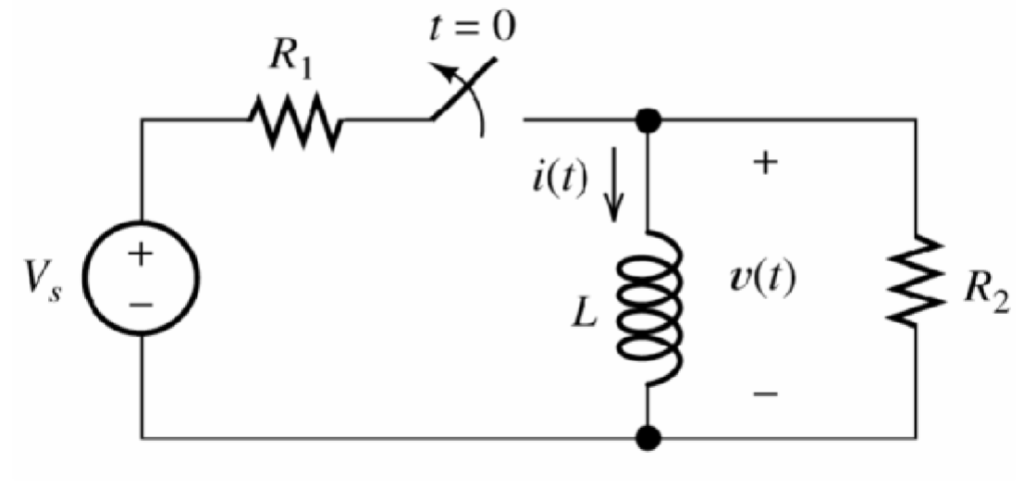
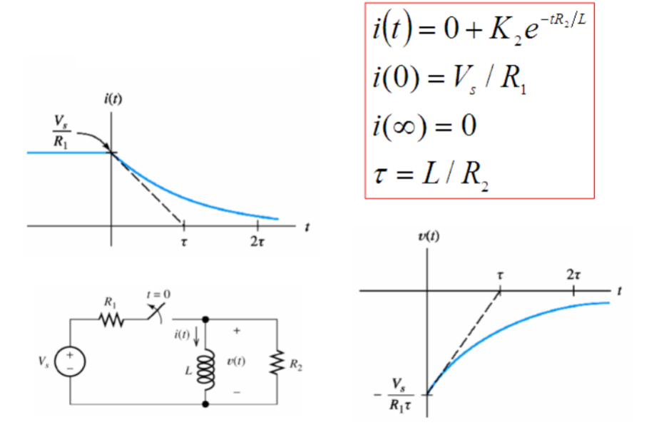
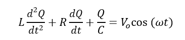
Steps for solving a for RL and RC Circuit

1. Apply Kirchhoff’s current and voltage laws to write the circuit equation (KCL, KVL).
   • Assume a solution of the form K₁ + K₂e^st.
2. Substitute the solution into the differential equation to determine the values of K1 and s .
3. Use the initial conditions to determine the value of K2.
4. Write the final solution.

Understanding Impedance

Now, don’t get scared by the word “impedance.” It’s just a fancy term that refers to the total opposition a circuit offers to alternating current (AC). It’s like the overall obstacle course for our electricity to overcome!

Impedance, often denoted by Z, is a complex number because it involves both resistance (R) and reactance (X). Reactance, in turn, depends on the frequency of the AC signal and the components in our RCL circuit.

Series RCL Circuits and Resonance

Let’s talk about two ways we can hook up our RCL components: series and parallel. We’ll start with series circuits.

In this setup, the impedance is just the sum of the individual impedance of the resistor, capacitor, and inductor. When we calculate the impedance at the resonant frequency, something magical happens! The reactance of the capacitor and inductor cancels out, leaving only the resistance behind.

Sample Problem

Solution

Parallel RCL Circuits and Resonance

In a parallel circuits the reciprocal of impedance (1/Z) is the sum of the reciprocals of the individual impedance of the resistor, capacitor, and inductor.

Again, when we hit that resonant frequency, the reactance of the capacitor and inductor becomes equal in magnitude but opposite in sign, leading to a super low impedance.

Sample Problem

Solution

Practical Applications of RCL Circuits and Resonance

Alright, you might be wondering, “Enough with the theory! How can we actually use this resonance thing?”

1. Filters: RCL circuits can act as fantastic filters. Depending on the frequency, they can either block certain signals (high-pass filters) or allow them to pass through (low-pass filters).
2. Tuners: Ever tuned a guitar or a radio? You’ve used resonance! RCL circuits can help us find the right frequency and fine-tune our instruments and radios to perfection.
3. Amplifiers: Resonance is also employed in certain amplifier circuits, helping boost specific frequencies and making your music sound awesome!

Designing RCL Circuits for Resonance

Alright, now comes the fun part – designing our very own RCL circuit for resonance! To do this, we need to consider a few things:

1. Choose the Components: Decide on the values of your resistor, capacitor, and inductor. Remember, the resonant frequency depends on these values, so choose wisely!
2. Calculate the Resonant Frequency: Use the formula we discussed earlier to find the resonant frequency for your chosen components.
3. Test and Tweak: Build the circuit and apply an AC signal with the calculated resonant frequency. Then, use an oscilloscope or other measuring tools to see if your circuit is resonating as expected. Tweak the values if needed to get that sweet resonance going!

Analyzing RCL Circuits with Resonance

Now that you’ve designed your circuit, let’s see how to analyze its behavior. When we hit the resonant frequency:

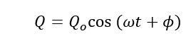
• Voltage Across Components: You’ll find that the voltage across the capacitor and inductor is equal but opposite in phase. At resonance, this voltage is at its maximum.
• Current Through Components: The current through the capacitor and inductor is also at its peak, making everything super lively!
• Power Factor: At resonance, the power factor of the circuit is unity, meaning the current and voltage are perfectly in phase.

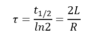
What is the time constant in RL and RC circuits?

The time constant in RL and RC circuits is a measure of how quickly the circuit reaches a steady-state condition or decays. The time interval Ƭ = RC is called the time constant of the circuit. In RL circuits, it represents the time it takes for the current to reach approximately 63.2% of its maximum value. In RC circuits, it indicates the time it takes for the voltage across the capacitor to reach 63.2% of its final value.

Conclusion

And there you have it, folks! We’ve explored the enchanting world of RCL circuits and discovered the power of resonance. From understanding the components to designing and analyzing our circuits, we’ve covered it all!

So go ahead, tinker with your circuits, and experience the magic of resonance for yourself. Whether you’re into music, electronics, or just love geeking out about cool science stuff, RCL circuits with resonance will surely spark your curiosity and creativity!

Sample Lab Report

Goals:

The goal of this experiment is to learn about RLC circuits and become familiar with the experimental aspect of resonance.

Procedure:

The Procedure used for this activity can be found on pp. 35-39 of the Phys 164 spring 2016 Lab Manual.

Measurements:

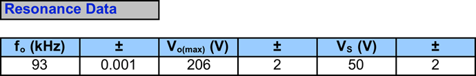
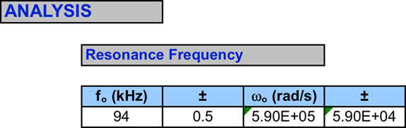
Analysis of Data:

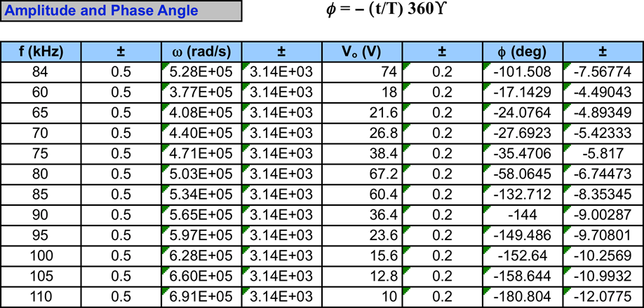
Results from tables:

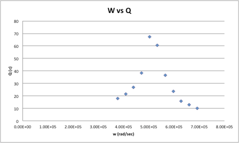
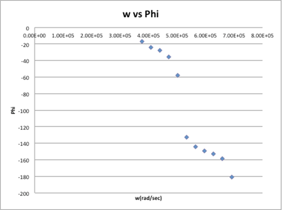
Graphs:

Calculations:

Conclusion:

The original values that were acquired for this experiment were extremely off and the data did not make much sense. Some of the possible sources of error are that the readings were taken by eyeballing the points of interest from the oscilloscope. This is not the most accurate way to take a reading, which could result in our values being so wrong. Also when looking for fo if the wrong data point was taken then the rest of the data would have been thrown off. The values for Vo were taken from another group to help make sense of the data acquired and have results, which could have been evaluated. After our data was fixed the shapes of both graphs more resemble the graphs in figure 19.2 on page 37. There is more resemblance between the graphs of Q vs W than the graph of W vs φ. In the graph, which shows W vs. f, there is an outlier at the last point (110khz), which appears at the bottom of the graph. The data for parts 1 and 2 do correlate, as there is an overlap between the tolerance zones. For the first part of the experimental angular frequency was 5.28×105 rad/sec while the expected value was 5.90×105 rad/sec. For the second part of the experimental angular frequency was 5.41×105 rad/sec while the expected value was 5.90×105 rad/sec.  This gave us a percent error of 8.2%. Both of these two parts have a relatively low %error with the first part having an 11% error and the second part having an 8% error.  In the final part of this experiment, the last angular frequency does not agree because the tolerance zones for these values did not overlap.