Kirchoff’s Voltage and Current Laws: Unraveling the Secrets of Voltage and Current in Circuits

Introduction

Today, we’re diving into the intriguing world of electrical circuits and uncovering the secrets behind Kirchoff’s Voltage and Current Laws. Now, you might be wondering why we need to understand these laws. Well, my friends, they form the very foundation of circuit analysis, helping us understand how voltage and current behave in circuits.

What are Kirchoff’s Voltage and Current Laws?

Alright, let’s start with the basics. Kirchoff’s Voltage Law (KVL) states that the algebraic sum of the voltages equals zero for any closed path (loop) in an electrical circuit. In simple terms, it means that the total voltage you gain in a loop is equal to the total voltage you drop.

On the other hand, Kirchoff’s Current Law (KCL) tells us that the sum of currents entering a node is equal to the sum of currents leaving that node. In simpler words, it’s like a traffic junction where the total incoming traffic is equal to the total outgoing traffic.

Kirchoff’s Voltage Law (KVL) in Action

Now, let’s see KVL in action. Imagine a circuit loop with resistors, batteries, and other components. KVL allows us to analyze and understand the voltage distribution across the circuit. We can apply it step-by-step, accounting for each voltage gain and voltage drop.

For example, if you have a circuit loop with a battery and resistors, you can use KVL to calculate the voltage drop across each resistor. By summing up these voltage drops, you can determine the total voltage of the battery.

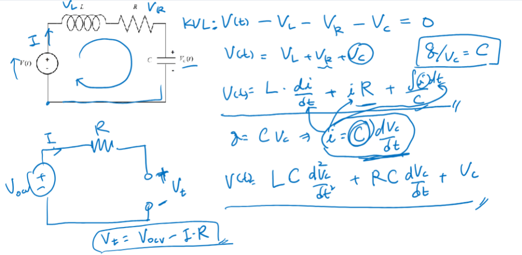
Sample Problem

Solve for the V_c & V_e in the system:

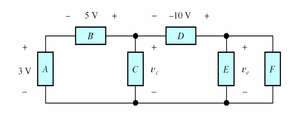
Solution:

Kirchoff’s Current Law (KCL) in Action

Moving on to KCL, this law helps us analyze the current flow in a circuit. Picture a node, which is like a junction point where multiple currents converge or diverge. KCL states that the net current entering a node is equal to zero. Alternatively the sum of currents entering a node equals the sum of the current leaving the node.

To understand this better, imagine a circuit with several branches connected to a single node. KCL allows us to calculate the current flowing through each branch. By applying KCL to the node, we can ensure that the total incoming current equals the total outgoing current.

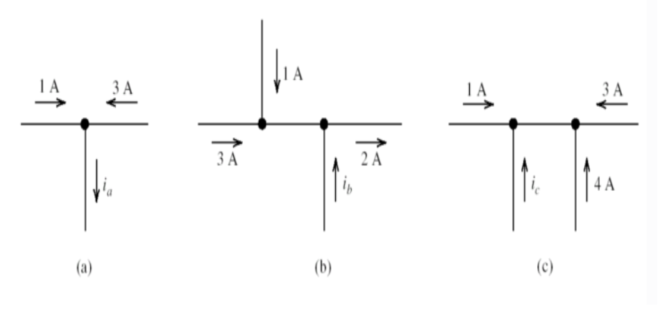
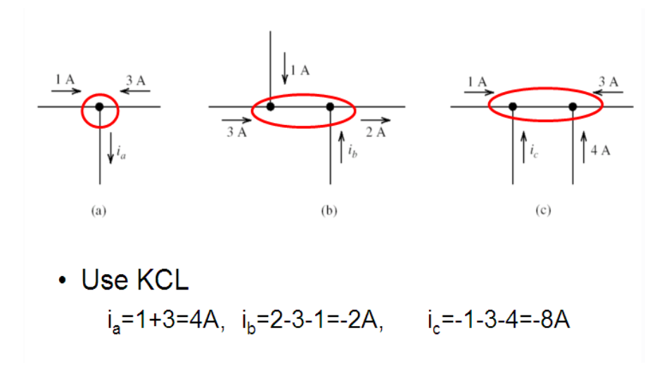
Sample Problem 1

Solve for the currents:

solution:

Sample Problem 2

Write the KCL equations in terms of node voltages:

Solution:

Sample Problem 3

Practical Tips for Applying Kirchoff’s Laws

Alright, now that we grasp the basic concepts, let me share some practical tips to make applying. Kirchoff’s laws a breeze. Trust me, these tips will save you from getting tangled up in complex circuit analysis!

1. Simplify the circuit: Start by simplifying the circuit as much as possible. Remove unnecessary components or combine resistors in series or parallel to reduce the complexity. The simpler the circuit, the easier it is to apply Kirchoff’s laws.
2. Assign direction and polarity: Assign a direction for current flow and a polarity for voltage across each component. Consistency is key here, so stick to your chosen directions and polarities throughout the analysis.
3. Label currents and voltages: Label the currents and voltages in the circuit diagram. This helps you keep track of what you’re analyzing and makes it easier to apply Kirchoff’s laws accurately.
4. Break it down: If you have a complex circuit with multiple loops or nodes, break it down into smaller parts. Analyze each loop or node separately using Kirchoff’s laws and then combine the results to get the overall solution.
5. Use algebraic equations: Convert the verbal expression of Kirchoff’s laws into algebraic equations. This allows you to solve for unknown currents or voltages using simultaneous equations. Remember to consider the signs (+/-) when writing the equations to account for voltage drops and gains.
6. Verify your solution: After solving the equations, verify your solution by checking if it satisfies Kirchoff’s laws. Ensure that the sum of voltages around any closed loop is zero and that the sum of currents entering and leaving each node is balanced.

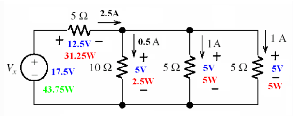
Sample Problem

Solve for Vx

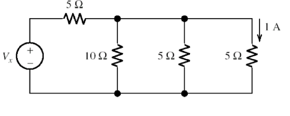
Step 1: Use KCL

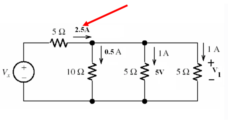
Step 2: Use KVL

Step 3: Power of Each Components

Sample Lab Report

Abstract:

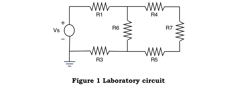
Using a breadboard and 6 resistors a circuit was constructed to confirm Kirchoff’s Voltage and Current Laws. A 10V-voltage was then connected to the circuit on the breadboard. See Figure 1 Laboratory circuit below. Using a multimeter, voltage and current measurements were taken across each resistor. These values were then compared to the algebraic results, which were computed using Kirchoff’s Voltage and Current Laws and Ohm’s Law.

Objective:

The purpose of this laboratory exercise was to confirm Kirchoff’s Voltage and Current Laws, within the range of voltage and current used in this experiment.

Theory:

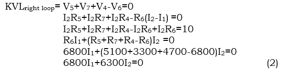
According to Kirchoff’s Voltage Law (KVL) the sum of the voltage inside a closed loop should always equal zero. If you look at the left loop of the circuit you get the following KVL equation. Assuming the current is traveling in the clockwise direction.

(1)                           KVL_{left loop}=-Vs+V₁+V₆+V₃=0

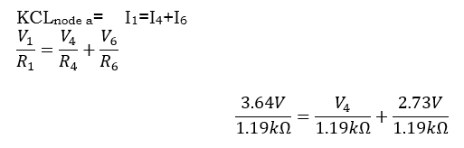
 Kirchoff’s Current Law (KCL) states that the sum of the current flowing into any node in a circuit must equal the sum of the current leaving that same node. If you name the junction located at the top center of the circuit in between R1, R4 and R6 as Node 1. And we assume I₁ is entering node 1 while I₄ and I₆ are leaving node 1, the following KCL equation can be derived.

(2)                                                      KCL_{node 1} = I₁=I₄+I₆

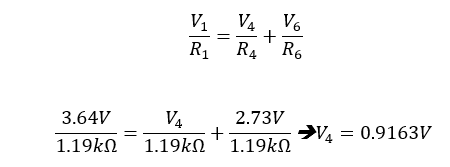
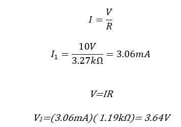
Using equation (2) you can then apply Ohms law which states that I=V/R to derive equation (3) which can be used in this example to solve for V₄, which is the voltage across R4.

(3)       

Procedure:

To simplify the experiment and the calculations all six resistors were picked of the same nominal resistance (1.2Ω). The first step in completing this experiment was to measure the actual resistance through each resistor using the multi-meter (1.19Ω). After the circuit was built as shown in Figure 1 Laboratory circuit, the multimeter was used to take voltage readings across each resistor. To get the current readings the multi-meter was connected in series to the resistor, which was being measured. After all the voltage and current values were recorded then the voltage and current values were calculated algebraically. To being to analyze this circuit, first, the circuit was simplified. Resistors connected in series can just be added together to find equivalent resistance.  

(4)                                                           R₄+R₇+R₅=R_a

1.19Ω+1.19Ω +1.19Ω =3.57kΩ

To find the equivalent resistance of two resistors connected in parallel you have to have to take the product of the two resistors and divide it by the sum of the two resistors.

(5)

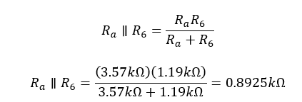
Using these two methods of circuit simplification you can simply the whole circuit to a voltage source and a single resistor of equivalent resistance (3.27Ω). By applying Ohms law you can then find the current through this simplified circuit, which is equivalent to the current flowing though the left loop of the circuit. Once you have the current flowing though the left loop you can find the voltage across both resistor 1 and resistor 3 by once again applying Ohms law.

(6)

Data and Analysis: The results from this experiment do confirm both KVL and KCL as the calculated currents and calculated voltages were very close to the actual current and voltage for the circuit. When comparing the measured and calculated results you see that all the calculated currents were within 2.6% of the actual value. This is a very low % difference, which just reinforces the validity of the results and KCL. To see a full list of all calculated currents see Table 1 measured vs calculated currents below.

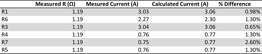
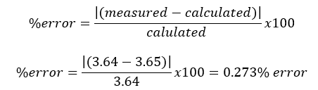
When comparing all the calculated voltages to the measured voltages the results show that the calculated voltage is within 0.66% of the actual voltage. This is an extremely low % difference, which proves that there is a very good correlation between these two values and reinforces the validity of the results. To see the full list of calculated voltages see Table 2 measured vs calculated voltages at the top of the following page.

Conclusions:

Table 1 of the previous section shows that the measured and calculated values of the current, agree to within 2.6%. Table 2 above shows that the measured and calculated values of voltages agree within 0.66%. see equation (7) below to see the sample calculation of % error

(7)

After performing this experiment it can be concluded that using KCL and KVL are valid methods for analyzing an electrical circuit.

Appendix

Equipment: Tektronix PS 280 DC Power Supply, Tektronix CDM 250 Digital Multimeter, 6 resistors with resistance values between 1kΩ-10kΩ, and a breadboard.

Pre-Laboratory Exercises:

Include these exercises in the laboratory report under a separate heading entitled, “Pre-laboratory Exercises” following the “Conclusion” section of the main report.

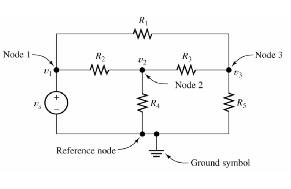
Referring to Figure 2 below:

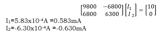
1. Using the given resistances and supply voltage, determine the indicated node voltages in Figure 1, using loop analysis and matrix solution methods. Show all your work.

Assume: left loop I₁ is traveling clockwise

Assume: left loop I₂ is traveling clockwise

Two equations two unknowns

2. Using the given resistances and supply voltage, determine the indicated node voltages in the Figure 1, using node analysis and matrix solution methods. Show all your work