Radial Heat Conduction

Abstract

The purpose of this lab was to determine the thermal conductivity k of the disk material by measuring the temperature distribution for transient and steady-state heat conduction in a cylindrical wall. To conduct this experiment cooling water was pumped though the HT10X Heat Transfer service Unit at approximately 1.5 liters/min. Initially the heating power of the system was set to 50%. The HT12 program read the temperature of all thermocouples every 10 seconds. After letting the power run for about 10 minutes the power was turned off for approximate 15 minutes.  This experiment was then repeated for heating power at 75% and 100%.  To determine the K value the following equation was used.

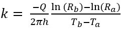
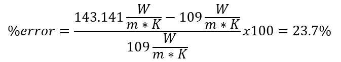
Where Q was the average heat power, T_bwas the temperature at the outer coupling, T_a was the temperature at the inter coupling, R_a was the inter radius R_b was the outer radius, h is the cylinder height. After preforming this experiment and averaging the three K values the average was found to be K_avg = 143.1 W/mK. The metal with the closest K value to the experimental value is magnesium, but due to its chemical properties it is unlikely the disk was this material. The second closest metal and most reasonable material for the disk to be made of is brass. Brass has a K value of 109 W/mK, which would result in 23% error. In engineering, thermal conductivity is important where heat transfer is of importance such as a heat exchanger or thermal insulator.

Experimental Results

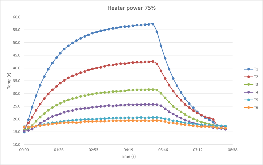
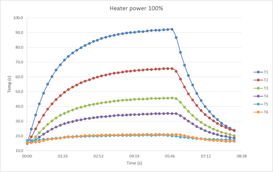
The experimental data extracted from the HT12 program for each of the heater powers tested was graphed in Figure 1 – Figure 3.

The measured steady state temperature values from Figure 1- 3 at each thermal coupling were then all converted to [K] in Table 1.  In the table R is the radius of each thermal coupling and ln(R) is the natural log of the radius of the coupling.

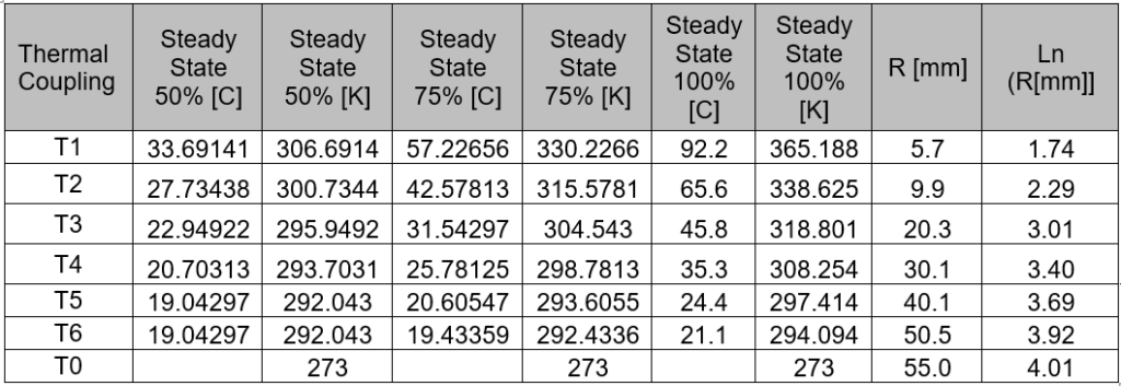
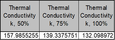
The values in Table 1 were then used to calculate the thermal conductivity value in Table 2 for each of the heating powers tested.

The data of Table 1 was used to create Figure 4, which graphs two curves:  one for the how the temperature of the thermal coupling changed with respect to the natural log of the radius of the coupling T(lnR) for 50% heating power,  and the other 100% heater power.

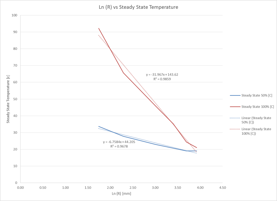
From the regression analysis, a statistically significant R² value of 0.9859 was found for the data set at 100% and the line of fit y = -31.967x +143.62 was obtained. Similar results were found at 50% of heater power with R² of 0.9678 and a line of fit of y = -6.7584x + 44.205. The statistically significant R² values support that Ln(R) and the steady state temperature are indeed directly proportional.

Based on the two equations found, T₀ at the outer periphery of the disk for 50% can be estimated to be 17.1 ^oC and T₀ at the outer periphery of the disk for 100% can be estimated to be 15.4 ^oC. There is a 16.38% difference between the K values for 50% and 100%.

Sample Calculations

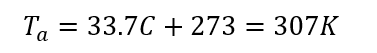
Temperature Conversion (K):

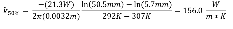
Thermal Conductivity (k):

% error: