The Reynolds Experiment
Background and Theory
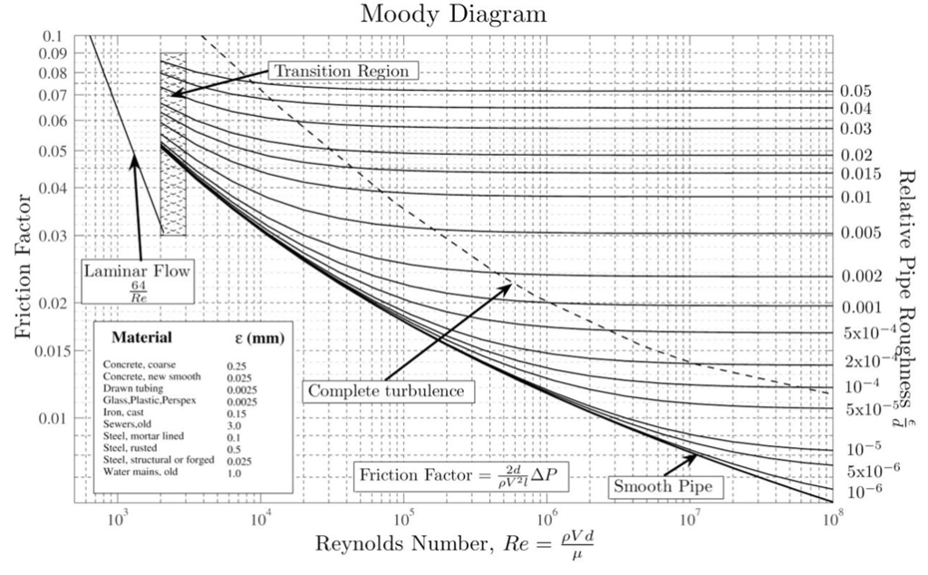
This laboratory aims to recreate the Moody diagram. Moody plotted the Moody Diagram in 1944, and it is now most famous and useful tool in fluid mechanics. The accuracy of the Moody chart is +/- 15 percent [1]. “The Moody Chart gives a good visual summary of laminar and turbulent pipe friction including roughness effects” [1].
The objective of this experiment is to experimentally recreate the Moody Chart, and to observe the transition from laminar to turbulent flow.
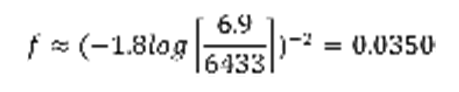
The experimental friction factor values are then going to be compared to the Haaland
Equation, which has a margin of error less than 2 percent [1].

(Eq. 1)
Where Re is the Reynolds Number, f is the friction factor, and ε/d is relative pipe roughness to diameter of pipe ratio.
Experimental Setup and Procedure
See Figure 1: Moody Diagram below. To begin this experiment you selected any size pipe. It was assumed that all pipes were smooth and there for had a relative pipe roughness of 0. The desired valve was then opened and the mass flow rate was calculated. Afterwards the pressure drop was then measured for that specific mass flow rate. Using the mass flow rate, the velocity of the fluid could be calculated using Eq.2.
Velocity (V):
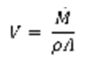
(Eq. 2)
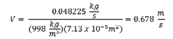
Where V was the velocity (m/s). M_dot is the mass flow rate (kg/s). ρ is the density of the fluid (kg/ m3). In this case the fluid used was water so: ρwater at 20oC : 998 kg/ m3 [1]. Finally A is the cross sectional area of the pipe tested (m2).
After the velocity of the water had been calculated the Reynolds Number was then found using Eq 3.

(Eq. 3)
Where Re # is the Reynolds Number. ρ is the density of water (kg/ m3). V is the average velocity of the fluid (m/s). d is the diameter of the pipe used (m). μ is the dynamic viscosity of the fluid (N s/m2). The fluid used was water so: μwater at 20oCis 1.002 x 10⁻³ N s/m2 [1].
Using the Reynolds number the theoretical friction factor could be calculated using Eq. 1 Haaland Equation from above. This friction factor was compared to the actual friction factor, which was calculated using Eq. 4.
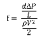
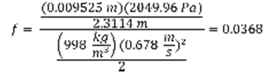
(Eq. 4)
where f is the experimental friction factor, d is the diameter of the pipe used (m), ρ is the density of water (kg/ m3), V is the velocity (m/s) and L is distance between measured points (m).
The experimental friction factor is then plotted against the Reynolds Number to recreate the Mood Diagram.
Experimental Results
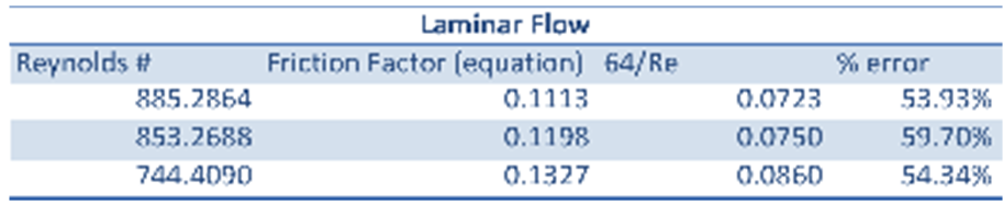
All experimental results are presented in the appendix. When comparing the experimental result to the theoretical result the trends are that the % error is much lower with the turbulent regime then the laminar regime. See Table 1: Turbulent Flow below and Table 2: Laminar Flow at the top of the following page.

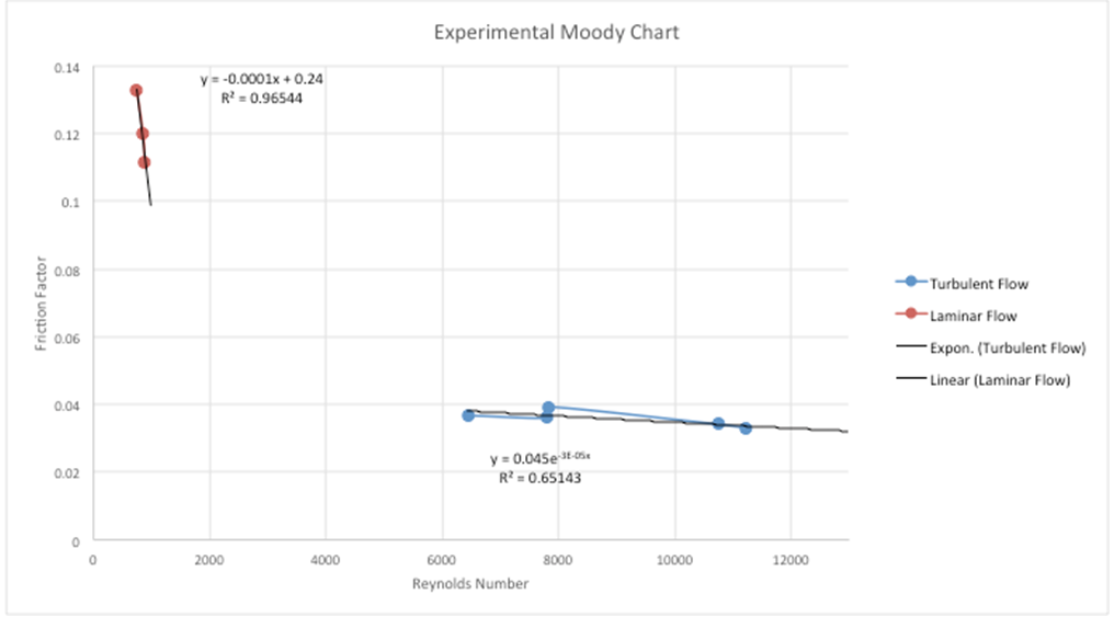
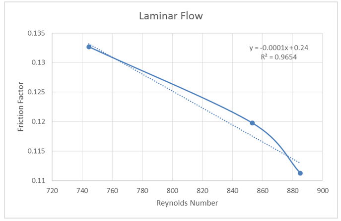
When this data was graph based off the Moody Diagram (Figure 1), the expectation was to see the laminar flow to linear resemblance line, meanwhile for turbulent flow the expectations were to see more of an exponential style graph. Even though the laminar flow had much higher % errors from theoretical the graph did resemble a linear line. One the other hand the turbulent flows had a much lower % error but due to the lack of range it was difficult to really see any shape to the curve. See Figure 2: Experimental Moody Chart below.
Discussion
Examining the data of Figure 2 one can see that the experimental Moody Chart is missing a large chunk. The lack of data points in the turbulent regime was due to the fact that when conducting this experiment you could only open the value so much while still being able to get pressure readings. If you exceeded the capacity of the system to read the pressure difference then you were not able to calculate the experimental friction factor. Even though that a complete moody diagram was not completed the turbulent did have much lower % errors ranging from 5.18% – 18.70% error. Where as the laminar flow had a much higher % error ranging from 53.93% – 59.70% . One of the reasons that this could have happened is due to the fact that with laminar flow the measured mass flow rate has a large impact in the accuracy of the results. When you are dealing with turbulent flows and larger mass flow rates some error in the technique calculating mass flow might have a small effect on your over all calculating. Where as when you are dealing with smaller flow rates the same error accumulates and results in a much larger error. The reason that the technique used to calculate mass flow rate is the most probably cause is because the errors in the laminar flow are very consistence. So even though the experimental friction factors were incorrect or had low precision they were very accurate. Another place this is low precision high accuracy of the laminar regime is seen, is when a linear regression was done the R2 value was 0.96 which indicates the values are represented well with a linear line. Some of the random error could be reduced by taking more than three repeats at each flow rate setting.
Conclusion
After conducting this experiment it is interesting to see how the friction factor has more of an effect in laminar regime instead of turbulent. This is believed to be cause because laminar flows tend to have a lower velocity there for they are more susceptible to the interior friction of the pipe.
Some things that could be changed to improve the results of this experiment is improve how the flow rates are calculated. Also if multiple trials were ran without changing the mass flow rate, then it could be easier to catch errors which are due to technique. If the range that pressure measurement could be taken also increased then it would have been easier to reproduce the moody diagram because the data points would be more spread out.
References
- F. M. White, Fluid Mechanics, 5th edition, , McGraw Hill, 2003
- J.P. Holman, Experimental Methods for Engineers, 7th Edition, McGraw Hill, New York, 2001
Appendix
Experimental Results

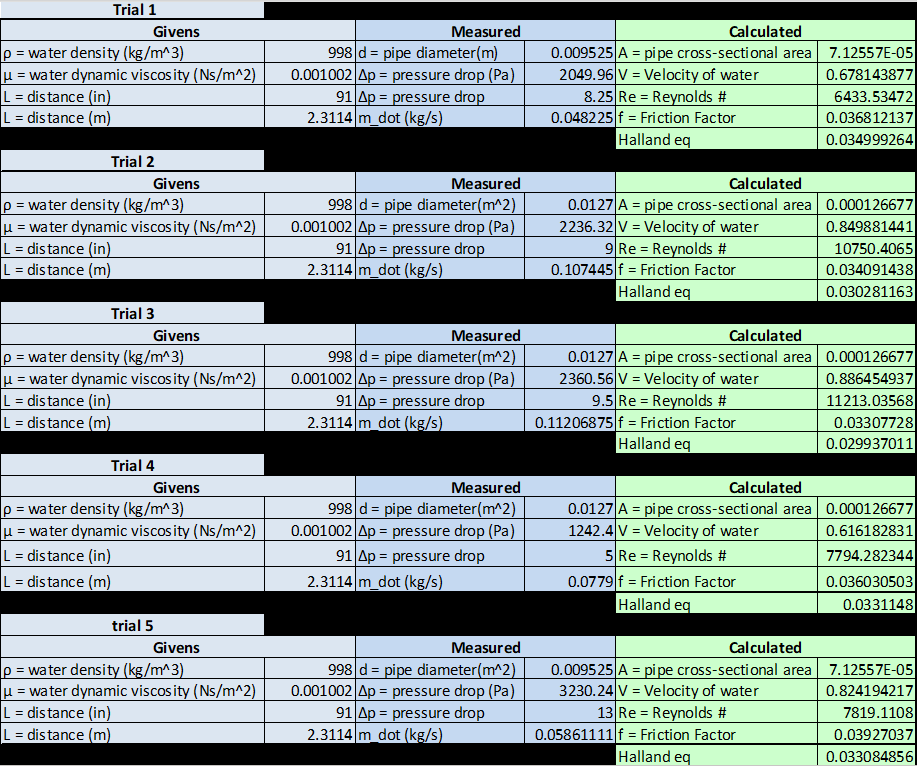
Sample Calculations:
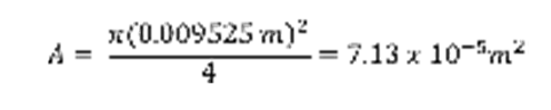
Area (A):
Velocity (V):
Reynolds Number (Re #):
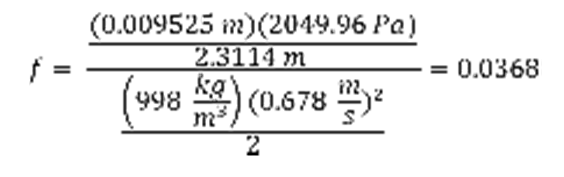
Friction Factor (f):
Haaland Eq (f):
% error: