Modeling of Dynamic Systems

In the realm of engineering and applied sciences, understanding and modeling dynamic systems are essential skills. When designing control systems, it is imperative to effectively model the dynamics of engineered systems. This model consists of a set of equations, typically differential equations, that depict the system’s dynamics based on the principles of physics. Through this model, one can analyze both the transient and steady-state performance of the system. This article delves into the mathematical modeling of dynamic systems, exploring concepts such as static vs. dynamic models, linear vs. nonlinear models, linearization, state-space representation vs. transfer function, and continuous- vs. discrete-time models.

Static vs. Dynamic Models

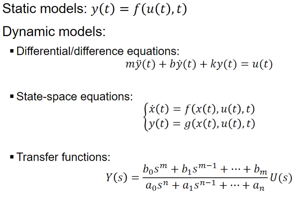
At the core of dynamic systems modeling lies the distinction between static and dynamic models. Static models describe the relationship between variables at a specific point in time, without considering their evolution over time. In contrast, dynamic models capture the temporal evolution of variables, taking into account how they change over time. Dynamic models are particularly useful for predicting future behavior or analyzing system stability.

Linear vs. Nonlinear Models

Dynamic models can further be classified into linear and nonlinear models based on the nature of their equations. Linear models exhibit a linear relationship between inputs and outputs, adhering to the principles of superposition and homogeneity. Simple linear models relate two variables (X and Y) with a straight line (y = mx + b). Transfer functions are generally linear.

Linearity→superposition holds

• If input 𝑢₁(𝑡) produces output 𝑦₁(𝑡) and input 𝑢₂(𝑡) produces output 𝑦₂(𝑡) ,
• Then 𝛼𝑢₁(𝑡) + 𝛽𝑢₂(𝑡) produces output 𝛼𝑦₁(𝑡) + 𝛽𝑦₂(𝑡) .

Nonlinear models, on the other hand, feature non-linear relationships, often resulting in more complex behavior. Nonlinear models relate the two variables in a nonlinear (curved) relationship

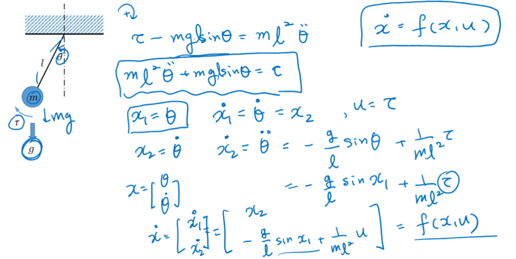
Example problem: Pendulum

Linear Systems:

In linear systems, the principle of superposition holds true, allowing us to calculate the response to a complex input by summing up the responses to its individual components. Linear Time-Invariant (LTI) Systems are characterized by being represented by lumped components and described by linear differential equations, with parameters that do not change with time. Systems where parameters vary over time are known as linear time-varying systems. Examples of linear time-varying systems include a car in motion or a rocket in flight, where the weight decreases as fuel is consumed.

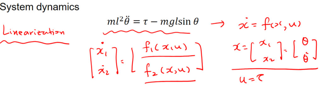
Linearization

Linearization is a technique used to simplify the analysis of nonlinear systems by approximating them as linear systems around an operating point. This is achieved by computing the first-order Taylor series expansion of the nonlinear equations. Linearization is particularly useful for analyzing system stability and designing control systems.

Most physical systems are nonlinear but linear systems are much better understood. A nonlinear system can be well approximated by a linear system in a ‘small’ neighborhood around a point in state space.

• Idea: Control keeps the system around some operating point (𝑥₀, 𝑢₀) → apply linearization around the operating point.

Linearization of Nonlinear Equations:

When a system operates briefly around an operating point, with minor variations about the equilibrium point, it is appropriate to approximate the system’s behavior using local linear approximations. This linearized Linear Time-Invariant (LTI) model is commonly used for designing controllers. By linearizing state and output nonlinear equations around a specific value of the state vector, we obtain Linear Time-Variant equations.

State-space Representation vs. Transfer Function

Two common approaches to representing dynamic systems are state-space representation and transfer function. State-space representation describes a system by a set of first-order differential equations, where the state variables represent the system’s internal state. State-space representations (or realizations) are not unique.

The transfer function, on the other hand, describes the system’s input-output relationship in the frequency domain, making it easier to analyze the system’s response to different inputs. In other words, the transfer function is a mathematical relationship between the input and output signals of the system

Example of State-space representations

Transfer Function:

The transfer function of a system defines the relationship between its input and output. It is denoted as G(s) and is a complex function that characterizes the system’s behavior in the s-domain, contrasting with the differential equations that describe its behavior in the time domain. The transfer function remains constant regardless of the input and does not reveal details about the system’s internal workings. Interestingly, the same transfer function can represent different systems.

One of the key benefits of the transfer function is its ability to calculate the output or response to various inputs. It can be derived analytically from the system’s physics equations or determined experimentally by observing the output for different known inputs.

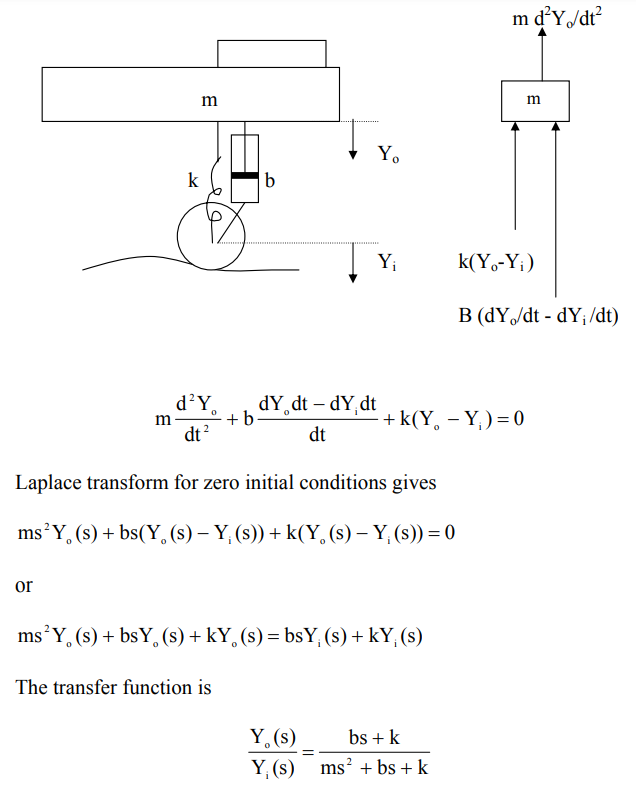
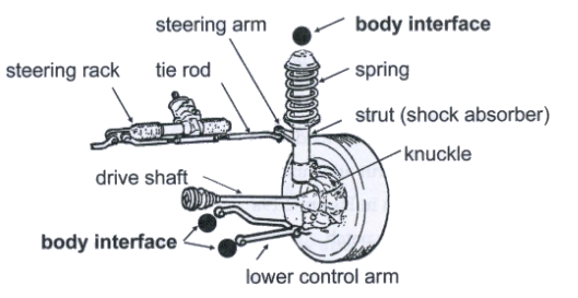
Example problem: Automotive Suspension System

State Space Representation

State-space control approaches emerged in Russia during the 1960s, known as Modern Control Theory, State Space Control Theory, or the Time Domain Approach, contrasting with Conventional Control Theory or Classic Control Theory, which adopts the Frequency Domain Approach.

A key limitation of conventional frequency domain models is their requirement for the system to be linear and Single Input Single Output (SISO).

Definitions:

• State Variables: These are the minimum variables needed to uniquely define the state of a dynamic system at any given moment.
• States: These are the values of the set of state variables. Given the current state values and input, the future state of the system can be calculated.
• State Vector: This refers to the vector containing all state variables.
• State Space: This is the hyperspace where the state of the system exists.

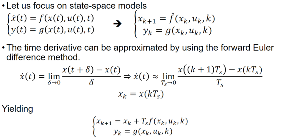
Continuous- vs. Discrete-Time Models

Dynamic systems can also be classified based on the nature of time representation: continuous-time and discrete-time models. Continuous-time models describe systems where the state variables change continuously over time, represented by differential equations. On the other hand, discrete-time models describe systems where the state variables change at discrete time intervals, represented by the difference equations.

Conclusion

Mathematical modeling of dynamic systems is a powerful tool that enables engineers and scientists to understand, analyze, and design complex systems. By understanding the distinctions between static and dynamic models, linear and nonlinear models, linearization techniques, and different representation methods, one can gain deeper insights into the behavior of dynamic systems. Whether designing control systems for autonomous vehicles or simulating the dynamics of biological systems, mastering the art of mathematical modeling is essential for tackling today’s complex engineering challenges.