Second-Order Electrical Circuits

Second-order electrical circuits play a crucial role in engineering and applied sciences, as they incorporate two energy storage elements—such as inductors and capacitors—along with resistors. Unlike first-order circuits, which contain only one energy storage element, second-order circuits exhibit both transient and steady-state responses, influencing electrical parameters like inductor current and capacitor voltage over time.

A common example of such circuits is the RLC circuit, which consists of resistors (R), inductors (L), and capacitors (C). These circuits are widely utilized in modeling and simulation applications, including battery cell behavior using Thevenin electrical circuit models. Additionally, their mathematical representation through the admittance function in the Laplace domain allows for precise analysis and calculation of circuit parameters. Due to their ability to model complex dynamic behaviors, second-order circuits are fundamental in various technological and scientific advancements.

Introduction to Second-Order Electrical Circuits

So, what are second-order electrical circuits, anyway? Well, in electronics, second-order electrical circuits involve components like resistors, capacitors, and inductors, which can create some pretty cool effects in a circuit. We often encounter these circuits in various electronic devices, audio equipment, and even in some parts of your car’s electronics.

Are second-order circuits and RCL circuits the same?

No, the second-order circuit and the RCL circuit are not the same. Second-order circuits are RLC circuits that contain two energy storage elements (inductor and capacitor). While an RC and RL circuit specifically denotes a circuit with only a resistor, capacitor, and/ or inductor. In other words, all second-order circuits are RCL circuits but not all RC and RL circuits are second-order circuits.

Understanding Differential Equations in Electrical Circuits

Now, don’t let the term “differential equation” scare you off. In plain English, it’s just a fancy way of describing how things change in a circuit over time. And trust me, it’s super useful in electrical engineering because it helps us understand how currents and voltages behave in different circuits.

Deriving Second-Order Differential Equations

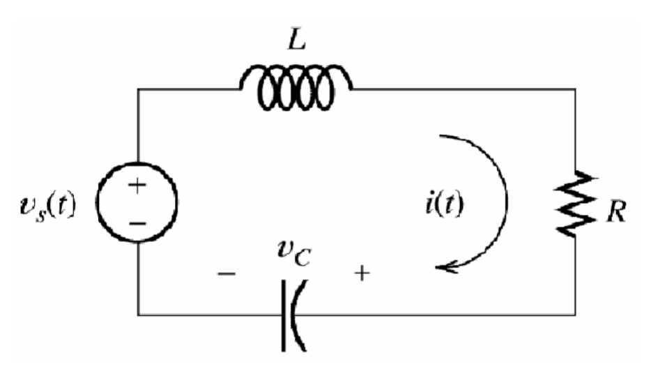
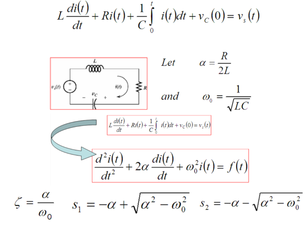
Alright, now it’s time to get a bit mathematical, but I promise it won’t be too scary. To derive second-order differential equations, we use Kirchhoff’s voltage and current laws – fancy names for some basic principles that describe how currents and voltages are distributed in a circuit. We’ll walk through the process step-by-step and even tackle a sample problem.

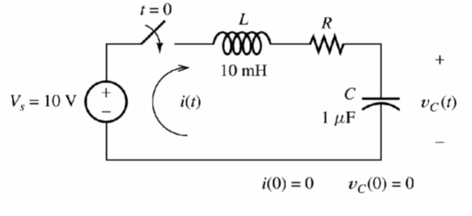
Sample Problem

Solution

Solving Second-Order Differential Equations

Once we’ve set up the equations, it’s time to solve them! There are different methods for this, like the homogeneous and non-homogeneous approaches. Oh, and keep an eye out for those time constants and damping – they play a vital role in understanding how the circuit behaves!

What is an overdamped circuit?

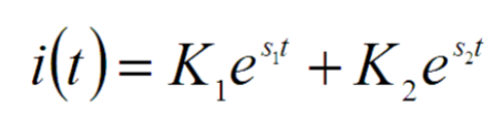
An over-damped circuit occurs when the damping factor is greater than 1 (ζ > 1 or equivalently, α > ω0). In this case, the circuit’s response to a disturbance is slow and gradual, without any oscillations. The current or voltage returns to its steady-state value without any overshoot or oscillatory behavior. The characteristic equations are real and distinct. The complementary solution is:

What is a critically damped circuit?

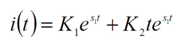
A critically damped circuit is a special case in second-order systems where the damping factor is exactly 1 (ζ = 1, or equivalently, α = ω0). It represents the fastest approach to equilibrium without any oscillations or overshoots. The system returns to its steady-state value as quickly as possible but without any oscillatory behavior. The roots are real and equal. The complementary solution is:

What is an underdamped circuit?

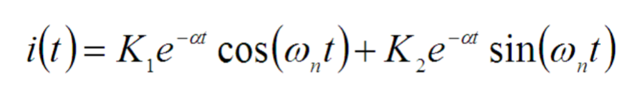
An underdamped circuit occurs in a second-order system when the damping factor is less than 1 (ζ < 1 or equivalently, α < ω0). It results in a decaying oscillatory response, where the current or voltage overshoots the steady-state value before settling down to it, leading to a series of damped oscillations. The roots are complex since they involve the square root of -1, in other words, the root forms are:

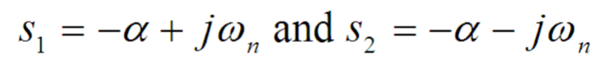
.The complementary solution is:

Application of Solutions to Second-Order Circuits

Alright, we’ve done the hard work and found solutions to our differential equations. But what does it all mean in the real world? We’ll see how circuits respond to different initial conditions and inputs. Plus, we’ll talk about how these concepts are applied in practical electronic devices and engineering projects.

Sample Problem

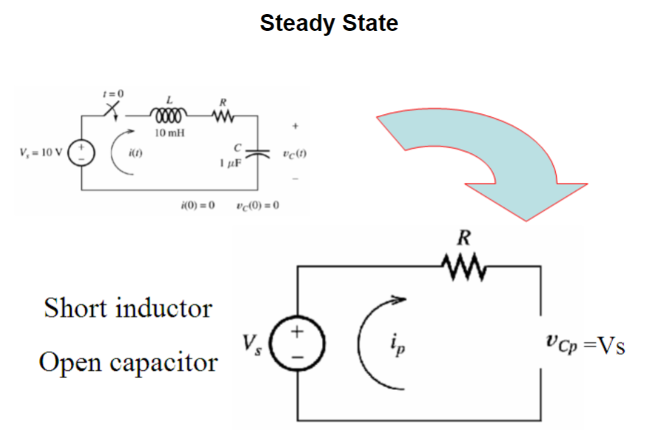
Step 1: Assume Steady State Circuit (short inductor and open capacitor)

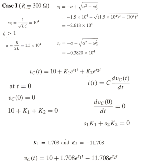
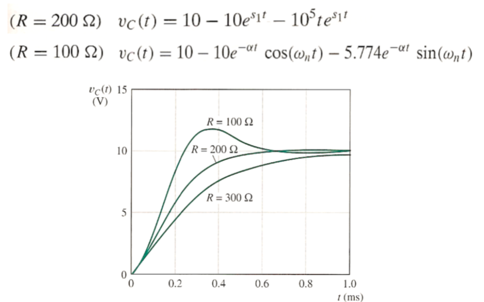
R = 300 Ohms: Solution

Solution (R = 100 and 200ohms)

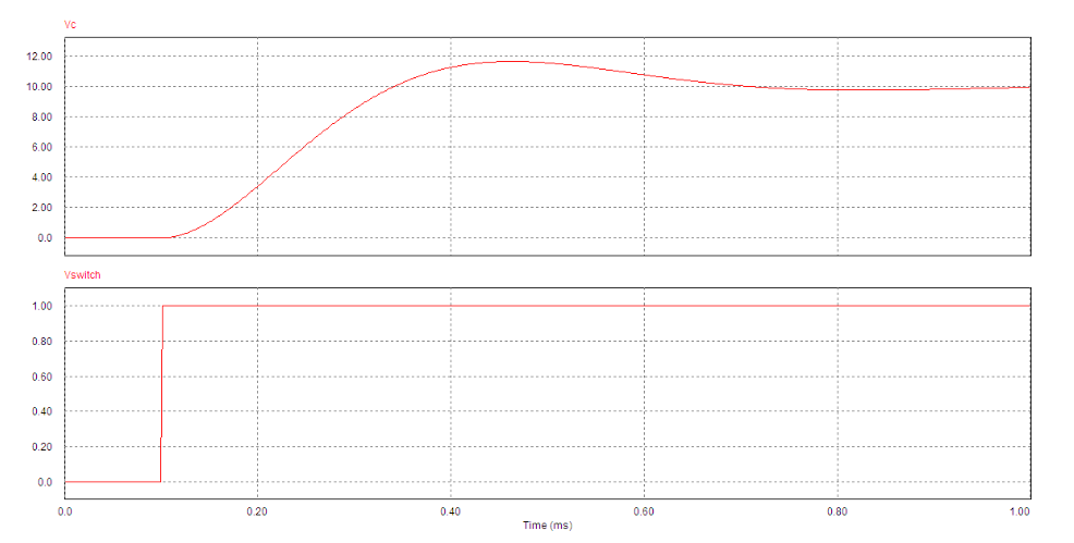
Example 2: RCL Circuits solved using online software such as PSIM

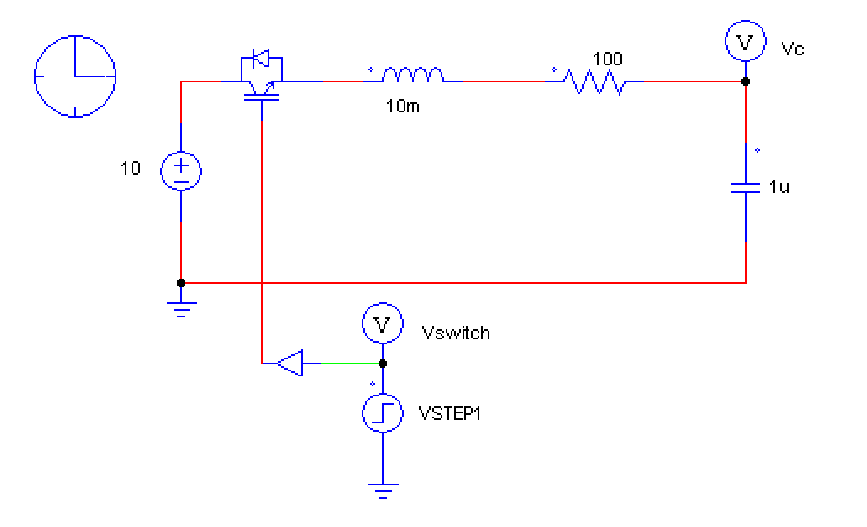
Results

Conclusion: Mastering Second-Order Circuits

So, there you have it, we’ve covered the basics of second-order electrical circuits and how to use differential equations to solve them. The world of electronics is vast and exciting, and understanding second-order circuits opens up a whole new realm of possibilities for us tech enthusiasts. So go ahead, tinker with some circuits, and let your creativity flow!

Remember, understanding second-order circuits and how to solve them using differential equations is an essential skill for anyone venturing into the field of electronics or electrical engineering. It gives you the power to design and analyze complex circuits, opening up doors to exciting opportunities and projects.

Thank you for joining me on this tech talk journey. Until next time, keep exploring, keep innovating, and keep being the brilliant, tech-savvy individuals that you are. Catch you later, my awesome circuit enthusiasts!