Full-wave Rectifier Circuit
Introduction
This report will examine the impact of adding two additional diodes to a full-wave rectifier circuit and the overall performance at varying engine speeds. The following sections will review the problem statement, key definitions, and background information, followed by the solution and conclusion.
Problem Statement
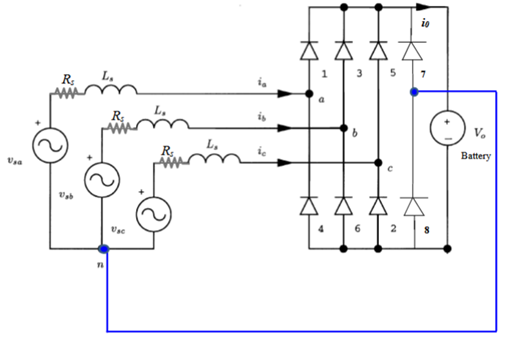
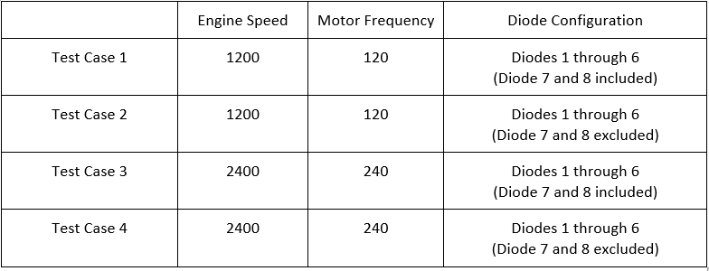
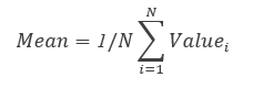
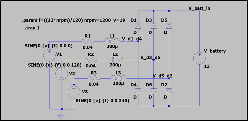
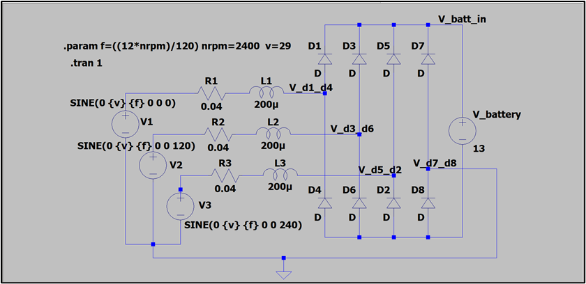
The circuit seen below in Figure 1.1 was provided as the premise of this project. The goal of this project was to determine the effects of removing Diodes 7 and 8 from the circuit shown below. The impact of eliminating the diodes will be examined for engine speeds of 1200 RPM and 2400 RPM to determine how engine speed influences the circuit.
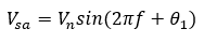
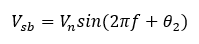
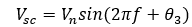
The given information was that Vsa , Vsb, and Vsc are sinusoidal 3-phase voltages offset 120° phase angles from each other. The frequency of the AC voltage can be represented by equation 1. a.
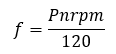
(1.a)
where f is the frequency, in Hz, P is the number of poles on the motor, and nrpm is the speed of the engine in RPM. Vo is a nominal 12V DC power source that can hold 14V when fully charged. There are three resistors Rs all 0.4 in series with three inductors Ls all with an inductance of 200 x 10-6H on each of the three-phase lines.
The frequency of the motor was assumed to be the same as the engine speed for this project. The following section will cover the general methods and techniques used to analyze this circuit.
The configurations tested and analyzed are as follows in Table 1.1 below. The following analysis will show the voltage, current, and power flow for each test case. In addition, we will show how we adjusted the magnitudes of Vsa , Vsb, and Vsc to achieve an 80A average current across the battery. Typically, the amplitude Vsa , Vsb, and Vsc were treated as equal. To round out the investigation, we examined the impact of Diodes 7 and 8 when at least one voltage is a different value.
Background
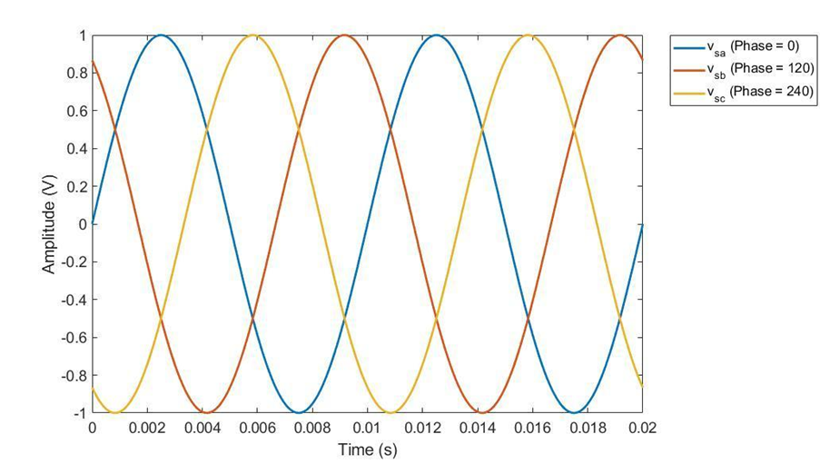
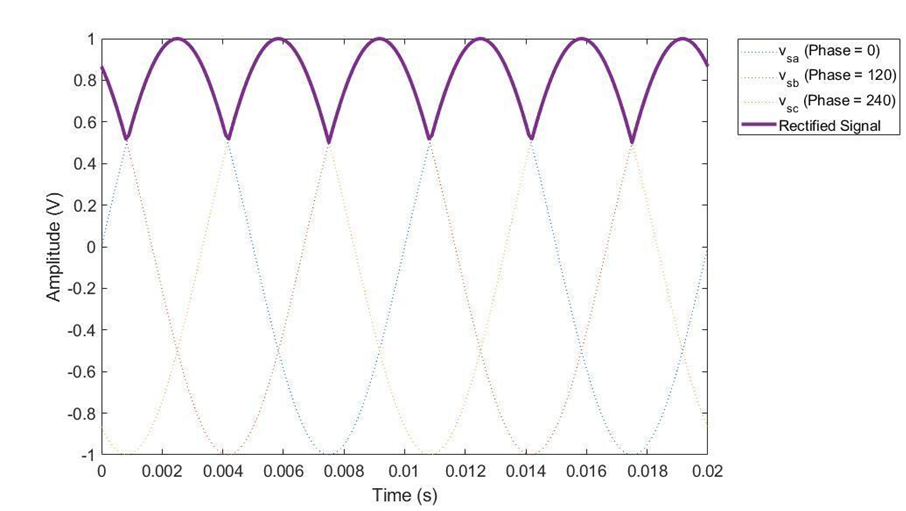
The circuit above is a model of a 3-sinusoidal voltage source with a full-wave rectifier and two additional diodes to prevent voltage spikes to the battery. This circuit consists of three AC voltage sources with 120-degree phase offsets, a DC battery, inductors, resistances, and diodes. Using a typical car as an example, the resistances, inductors, and AC voltage supplies represent the alternator; while the diodes represent the rectifier that converts the AC voltage into a DC voltage that can be absorbed by the DC battery. Figure 1.2 depicts an AC voltage supply and the equations for the plotted lines are shown in Equations 1.b, 1.c, and 1.e.
(1.b)
(1.c)
(1.e)
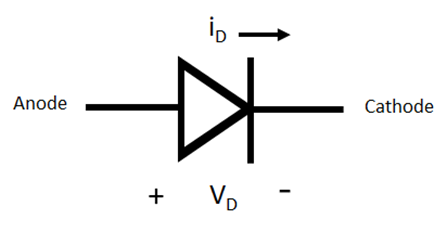
At its most basic, diodes are used to control the direction of current flow, similar to a check valve in a hydraulic or pneumatic system that allows fluid to flow in one direction. Diodes only allow current to pass when the voltage across the diode is positive, and the flow of the current moves from the anode to the cathode as shown in Figure 1.3. The characteristics of an ideal diode are outlined in Table 1.2 and depicted in Figure 1.4.
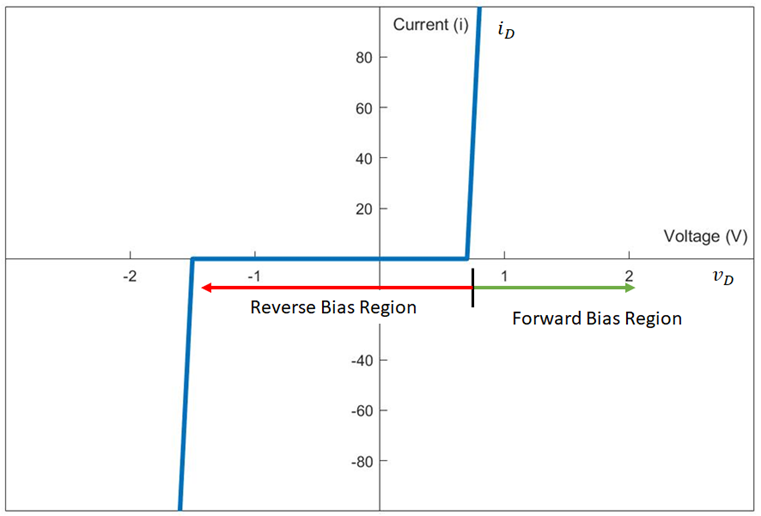
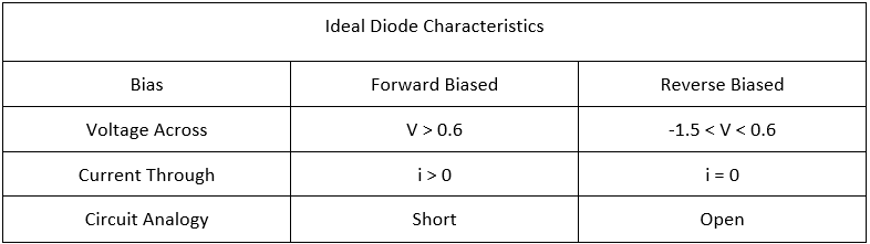
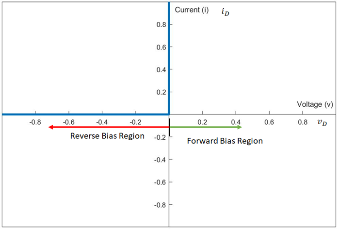
In order to simplify calculations for the larger more complex circuits, we often model diodes using the ideal diode model with the current-voltage characteristic as shown in Figure 1.5. Throughout this report, we modeled all diodes as ideal diodes.
The configuration of Diodes 1 through 6 constitutes a full rectifier in the problem statement (Figure 1.1). The benefit of using a full rectifier is that we can take the waveforms as shown in Figure 1.2 and transform them to the single output voltage from the rectifier shown in Figure 1.6 below. This voltage acts as a DC voltage and can be absorbed by the DC battery on the right side of Figure 1.1.
Power is defined as the product of current and voltage, as shown in Equation 1.f. Power is typically expressed in units of Watts.

(1.f)
There are several ways to calculate the average of instantaneous values. For purposes of this report, a simple vector average was computed by use of MATLAB’s mean() function. This is a simple function that considers all data points rather than a rolling average. The core equation used for the mean() is shown in Equation 1.g.
(1.g)
Simulation Development and Assumptions
LTspice was used to develop four models, one for each circuit scenario given in the problem statement. The model layout is shown below; also included in the Appendix are the raw files so the results can be replicated. The LTspice and Simulink simulation assume the diodes to be ideal. The voltage loss across them is assumed to be negligible; therefore the increased complexity of simulating non-ideal diodes would add little value.
This simulation assumes 13V for the battery voltage to approximate a window of time part-way through the battery’s charging cycle. Assuming a “midpoint” of the battery’s normal operating range is suitable for an overall understanding of the system behavior. If a more detailed understanding is required, a more advanced battery model should be developed and used as discussed in Section 3.4. Due to this assumption, the model output is most relevant for a small time window. Accordingly, the LTspice simulation was performed for 1s.
Finally, it is also assumed that the transient circuit behavior is not of interest, only the steady-state operation. To this end, although the simulation does include the initial transient behavior, the data shown later in this report is selected after a sufficiently long simulation time to only represent the steady-state behavior expected. Figures 2.1 to 2.4 below show the exact model setup used to obtain the output shown later in this report. Figure 2.5 shows the Simulink model setup used to obtain the solution in Section 3.4 with a more advanced lead-acid battery model.

Varied Input frequency
When varying the input frequency, the overall system behavior is very similar. Comparing the waveforms in Figures 2.5 and 2.7, a minimal difference is noted. The most obvious change is of course the increased frequency of the waveforms due to the increased input engine speed. However, when the engine is spinning at 2400 RPM, about 29V is needed to generate the 80A battery input specified. When the engine is spinning at 1200 RPM, only about 19V is needed to generate approximately the same input amperage.
The difference in voltage needed to achieve 80A battery input can be explained by the fact that the impedance of the inductors (L1, L2, and L3) increases proportionally with the frequency according to the formula ZL = j⍵L where ⍵=2𝝅ƒ. Thus, a higher voltage is needed to overcome the impedance to result in the same current at the battery input per Ohm’s Law.
Graphical Simulation Output
Figures 2.5 to 2.8 show the output of the simulation. As discussed in Section 2.1, these plots show the behavior at steady-state.
Diode States with Equal Voltages
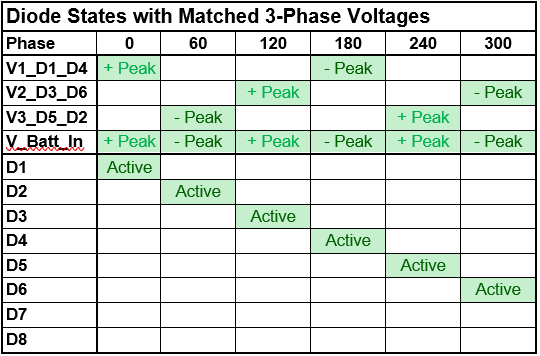
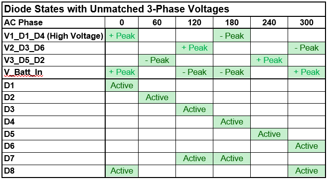
When the 3-phase sinusoidal input voltages were equal, diode states were easily predictable based on the positive and negative peaks of each sinusoidal voltage waveform. When the waveforms are at their positive peak, current flows through the “forward” bias Diodes, 1, 3, and 5. When the waveforms are at their negative peak, current flows through the “reverse” bias Diodes, 2, 4, and 6. Table 2.1 illustrates the state of each diode based on the phases, positive peaks, and negative peaks.
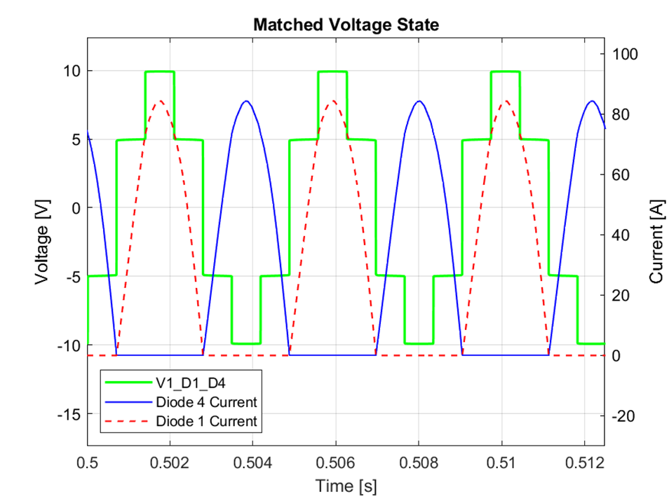
Figure 2.11 illustrates the principle by graphing one voltage input V1_D1_D4 with the currents of Diodes 1 and 4. Diode 1 was the “forward” bias diode, and Diode 4 was the “reverse” bias diode. When the sinusoidal voltage V1_D1_D4 is at its positive peak, Diode 1 allows current to flow through to the battery’s positive side, and Diode 4 blocks current flow to the battery’s negative terminal. When the sinusoidal voltage V1_D1_D4 is at its negative peak, Diode 4 allows current to flow from the battery’s negative terminal, and Diode 1 blocks current flow from the battery’s positive terminal. The behavior between the circuit’s other sinusoidal voltage and diode sets match the described behavior, but at different phase angles.
With equal sinusoidal voltages, Diodes 7 and 8 are never active. Additionally removing Diode 7 and 8 does not change the behavior of the rest of the circuit.
The Diode States With Unequal Voltages
The behavior of the circuit changes when the voltage of one phase does not match the voltage of the other two phases. When the voltages are unmatched, Diodes 7 and 8 will become active. Their activation follows the waveform of the voltage V_Batt_In.
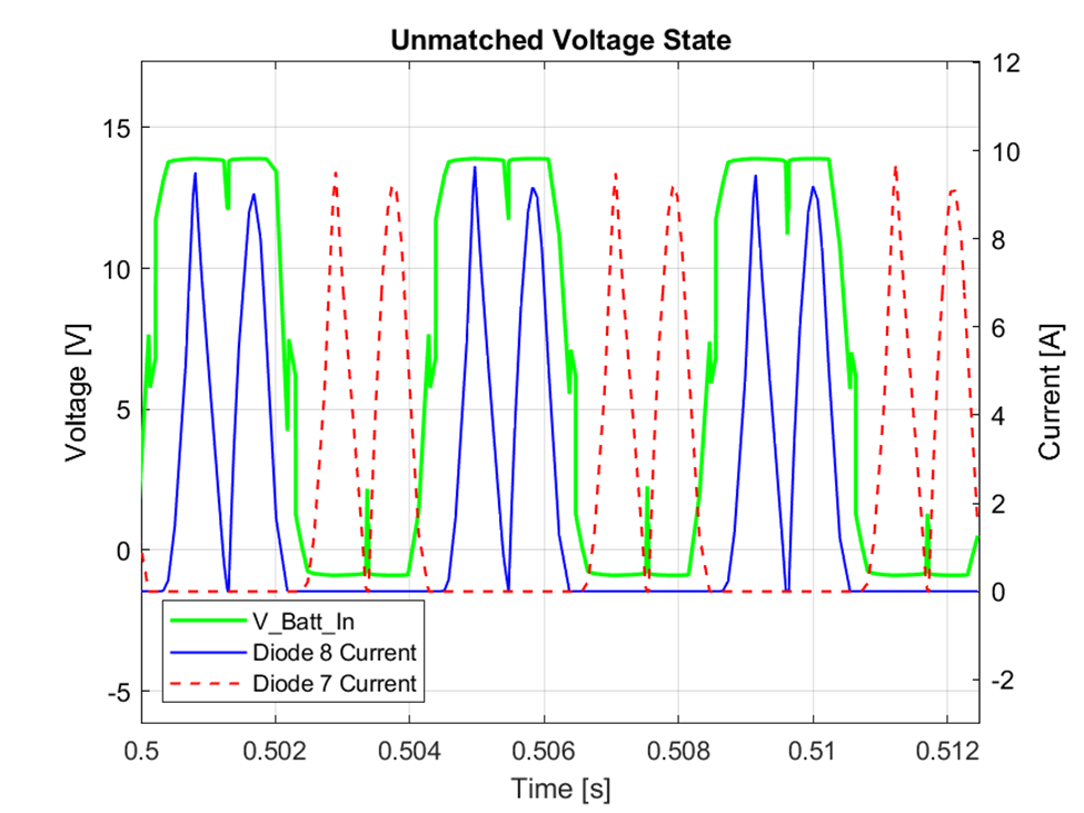
Figure 2.12 illustrates what this looks like by graphing the voltage V_Batt_In with the currents of Diodes 7 and 8. Diode 7 is the “forward” bias diode and allows current to flow from the ground reference to the battery’s positive terminal when the voltage V_Batt_In reaches its negative peaks. Diode 8 is the “reverse” bias diode and allows the current to flow from the battery’s negative terminal to ground reference when the voltage V_Batt_In reaches its positive peaks.
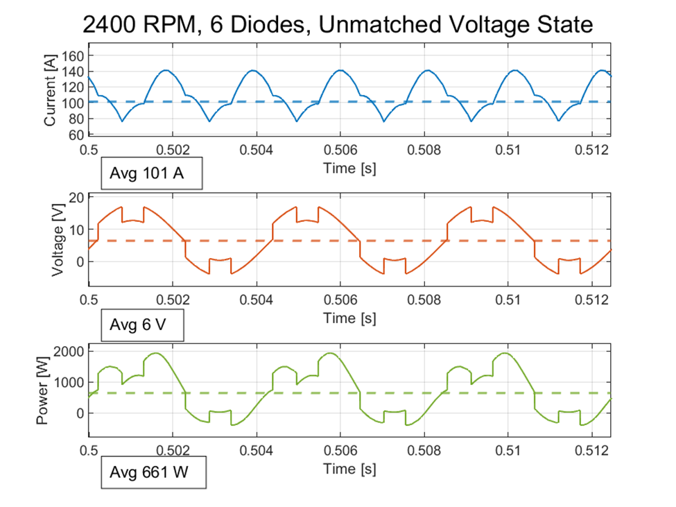
With and Without Diodes 7 and 8 With Unequal Voltages
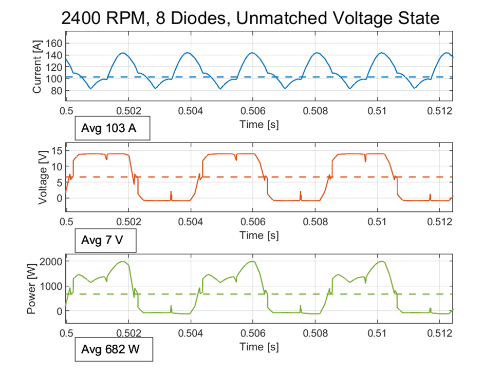
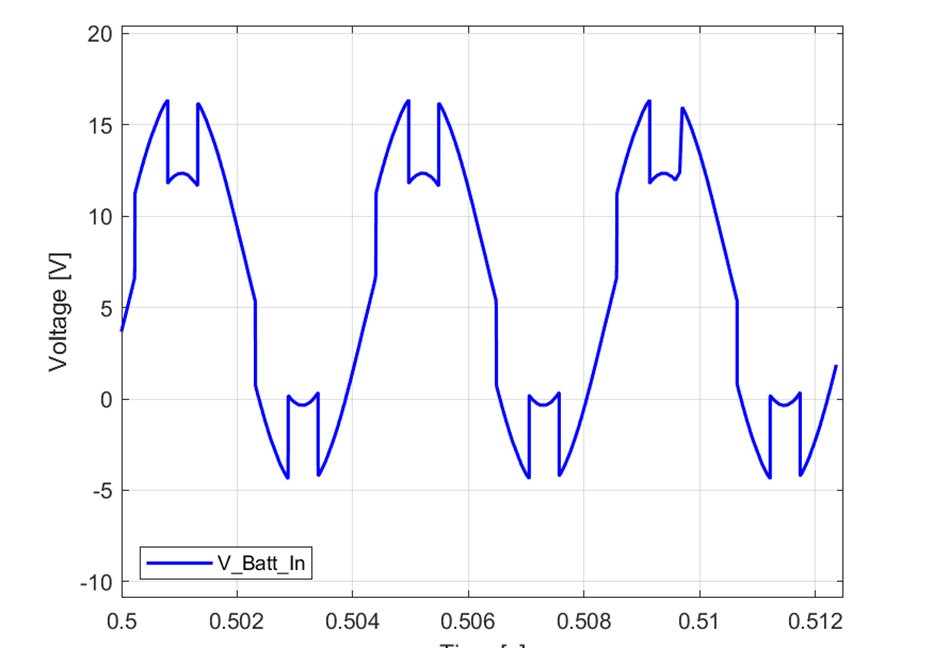
When one of the 3-phase input voltages does not match the other two phases, removing Diodes 7 and 8 has an effect on the circuit. Specifically, it affects the voltage peaks that the battery is exposed to. Figure 2.13 shows the voltage V_Batt_In waveform with Diodes 7 and 8 removed. Peak voltages are around 17V compared to peak voltages of 14V in Figure 2.12 where Diodes 7 and 8 are present.
Considering the nominal operating range of the battery is stated to be between 12V and 14V, there is a risk that the battery could be exposed to a damaging level of voltage with Diodes 7 and 8 removed.
Additionally, incrementally more power can be delivered to the battery when Diodes 7 and 8 are present. In the specific scenario examined, Figures 2.9 and Figure 2.10 show approximately a 3% increase in average power delivered to the battery. While the scenario examined was not likely more extreme than would occur in a real system, the voltages will never perfectly match.
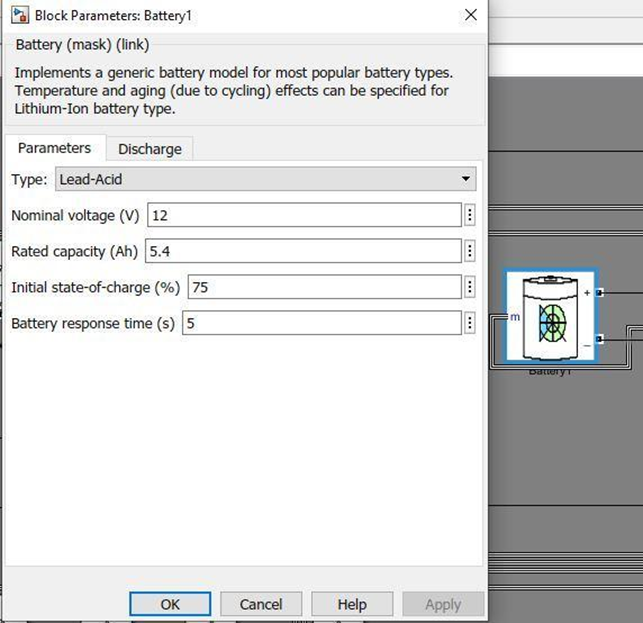
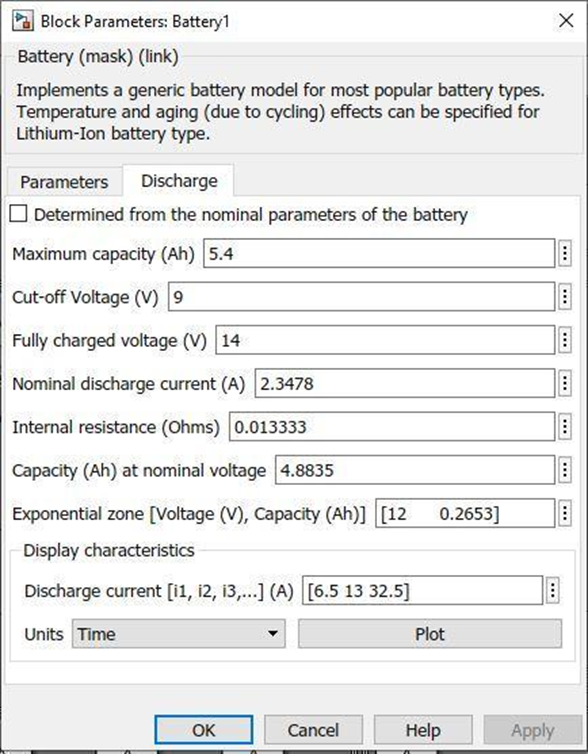
Implementing a Lead Acid Battery Model and 3-Phase Breaker
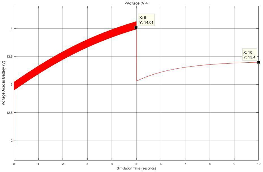
Figure A1 in the appendix shows a Simulink model implementing a real lead acid 12V battery model and a 3-phase breaker to separate the AC power sources from the rectifier and battery. The purpose of this is to compare the ideal 12V voltage source results given by the experiment with that of a real lead acid battery which, presumably, would behave slightly differently when charging and discharging. The 3-phase breaker was added to observe the battery’s behavior in this circuit when power was not being supplied.
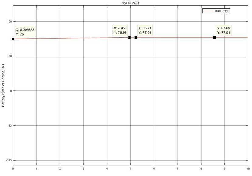
Figure 2.13 shows the voltage versus time plot of the above simulation over a 10s period, where the 3-phase breaker was opened at t=5s effectively cutting power to the battery/charging circuit. the initial state of charge of the battery was set to 75%, and a nominal voltage of 12V. Figure 2.13 shows the voltage rising in a somewhat logarithmic curve while the battery is charging, then dropping suddenly when the switch is opened. and leveling off again.
Figure 2.14 shows the state of charge over time of the same circuit. It can be seen that the battery SOC starts at 75%, then rises to 77.01% before the switch opens at t=5 seconds. After this time, the battery maintains its current state of charge for the remainder of the simulation.
This is because the only way the battery could discharge in this circuit if is Diode 8 was on, and given the voltage of the inputs/battery, this diode remains off and thus current can only flow within the rectifier/battery loop. This also explains why removing Diodes 7 and 8 had no effect since it can be shown that Diode 8 has zero current across it and thus is not on at these voltages. The setup for the battery model is also shown below in Figures A2 and A3.
Conclusion
For a real-world circuit with inherent voltage variations, the model output and analysis result in a recommendation to retain Diodes 7 and 8 for this system. These diodes both serve to shield the battery from input voltage spikes, and to maximize power delivery in scenarios where the 3-phase voltages are not equal. However, in the ideal case, where all 3-phase voltages have the same amplitude, as initially laid out in this project scope, Diodes 7 and 8 have no effect on the circuit.
Appendix
Appendix A: Lead acid battery model layout and battery specifications
Appendix B: LTSpice Models Used
Version 4
SHEET 1 880 680
WIRE 80 -16 0 -16
WIRE 160 -16 80 -16
WIRE 240 -16 160 -16
WIRE 320 -16 240 -16
WIRE 0 32 0 -16
WIRE 80 32 80 -16
WIRE 160 32 160 -16
WIRE 240 32 240 -16
WIRE -304 144 -464 144
WIRE -176 144 -224 144
WIRE -32 144 -96 144
WIRE 0 144 0 96
WIRE 0 144 -32 144
WIRE -464 176 -464 144
WIRE 320 192 320 -16
WIRE -288 240 -400 240
WIRE -160 240 -208 240
WIRE 64 240 -80 240
WIRE 80 240 80 96
WIRE 80 240 64 240
WIRE -400 272 -400 240
WIRE 240 320 240 96
WIRE 256 320 240 320
WIRE 400 320 256 320
WIRE -272 336 -336 336
WIRE -144 336 -192 336
WIRE 128 336 -64 336
WIRE 160 336 160 96
WIRE 160 336 128 336
WIRE -336 368 -336 336
WIRE 0 368 0 144
WIRE 80 368 80 240
WIRE 160 368 160 336
WIRE 240 368 240 320
WIRE -336 384 -336 368
WIRE 0 480 0 432
WIRE 80 480 80 432
WIRE 80 480 0 480
WIRE 160 480 160 432
WIRE 160 480 80 480
WIRE 240 480 240 432
WIRE 240 480 160 480
WIRE 320 480 320 272
WIRE 320 480 240 480
WIRE -464 496 -464 256
WIRE -400 496 -400 352
WIRE -400 496 -464 496
WIRE -336 496 -336 448
WIRE -336 496 -400 496
WIRE 160 496 160 480
WIRE -400 528 -400 496
WIRE 400 528 400 320
WIRE 400 528 -400 528
FLAG 320 -16 V_batt_in
FLAG 64 240 V_d3_d6
FLAG -32 144 V_d1_d4
FLAG 128 336 V_d5_d2
FLAG 256 320 V_d7_d8
FLAG 160 496 0
SYMBOL diode 16 96 R180
WINDOW 0 24 64 Left 2
WINDOW 3 24 0 Left 2
SYMATTR InstName D1
SYMBOL diode 176 432 R180
WINDOW 0 24 64 Left 2
WINDOW 3 24 0 Left 2
SYMATTR InstName D2
SYMBOL diode 96 96 R180
WINDOW 0 24 64 Left 2
WINDOW 3 24 0 Left 2
SYMATTR InstName D3
SYMBOL diode 16 432 R180
WINDOW 0 24 64 Left 2
WINDOW 3 24 0 Left 2
SYMATTR InstName D4
SYMBOL diode 176 96 R180
WINDOW 0 24 64 Left 2
WINDOW 3 24 0 Left 2
SYMATTR InstName D5
SYMBOL diode 96 432 R180
WINDOW 0 24 64 Left 2
WINDOW 3 24 0 Left 2
SYMATTR InstName D6
SYMBOL diode 256 96 R180
WINDOW 0 24 64 Left 2
WINDOW 3 24 0 Left 2
SYMATTR InstName D7
SYMBOL diode 256 432 R180
WINDOW 0 24 64 Left 2
WINDOW 3 24 0 Left 2
SYMATTR InstName D8
SYMBOL ind -192 160 R270
WINDOW 0 32 56 VTop 2
WINDOW 3 5 56 VBottom 2
SYMATTR InstName L1
SYMATTR Value 200µ
SYMBOL ind -176 256 R270
WINDOW 0 32 56 VTop 2
WINDOW 3 5 56 VBottom 2
SYMATTR InstName L2
SYMATTR Value 200µ
SYMBOL ind -160 352 R270
WINDOW 0 32 56 VTop 2
WINDOW 3 5 56 VBottom 2
SYMATTR InstName L3
SYMATTR Value 200µ
SYMBOL res -208 128 R90
WINDOW 0 0 56 VBottom 2
WINDOW 3 32 56 VTop 2
SYMATTR InstName R1
SYMATTR Value 0.04
SYMBOL res -192 224 R90
WINDOW 0 0 56 VBottom 2
WINDOW 3 32 56 VTop 2
SYMATTR InstName R2
SYMATTR Value 0.04
SYMBOL res -176 320 R90
WINDOW 0 0 56 VBottom 2
WINDOW 3 32 56 VTop 2
SYMATTR InstName R3
SYMATTR Value 0.04
SYMBOL voltage -464 160 R0
WINDOW 0 35 49 Left 2
WINDOW 3 -129 5 Left 2
WINDOW 123 0 0 Left 0
WINDOW 39 0 0 Left 0
SYMATTR InstName V1
SYMATTR Value SINE(0 {v} {f} 0 0 0)
SYMBOL voltage -400 256 R0
WINDOW 0 39 54 Left 2
WINDOW 3 -176 9 Left 2
WINDOW 123 0 0 Left 0
WINDOW 39 0 0 Left 0
SYMATTR InstName V2
SYMATTR Value SINE(0 {v} {f} 0 0 120)
SYMBOL voltage -336 352 R0
WINDOW 0 42 52 Left 2
WINDOW 3 9 98 Left 2
WINDOW 123 0 0 Left 0
WINDOW 39 0 0 Left 0
SYMATTR InstName V3
SYMATTR Value SINE(0 {v} {f} 0 0 240)
SYMBOL voltage 320 176 R0
WINDOW 123 0 0 Left 0
WINDOW 39 0 0 Left 0
SYMATTR InstName V_battery
SYMATTR Value 13
TEXT -608 32 Left 2 !.param f=((12*nrpm)/120) nrpm=2400  v=29
TEXT -592 72 Left 2 !.tran 1
Appendix B: MATLAB Script Used
%Performs calculations for plot generation for ECE 510 Project #2 ---------
% Credit: https://github.com/PeterFeicht/ltspice2matlab (called in script)
%Setup - Initial commands -------------------------------------------------
clearvars; clc; clf;
vecAmpColor = [0 0.447 0.741];
vecVoltColor = [0.85 0.325 0.098];
vecPowerColor = [0.467 0.675 0.188];

% Pull in LTSpice data and plot 2400 RPM, 8 Diode Variant -----------------
[LTS2400r8dTime,LTS2400r8dBattAmp, LTS2400r8dTimeChop, LTS2400r8dBattAmpChop] =...
    fxnGetLTSpiceData('project2_2400r8d.raw','I(V_battery)', 0.500, 0.5125);
[~,LTS2400r8dVbatt, ~, LTS2400r8dVbattChop] =...
    fxnGetLTSpiceData('project2_2400r8d.raw','V(v_batt_in)', 0.500, 0.5125);
calcPwr2400r8d = LTS2400r8dVbatt .* LTS2400r8dBattAmp; % power = V*A
calcAvg2400r8dVbatt = mean(LTS2400r8dVbatt,'omitnan');
calcAvg2400r8dBattAmp = mean(LTS2400r8dBattAmp,'omitnan');
calcAvg2400r8dPwr = mean(calcPwr2400r8d,'omitnan');
axisY1min = min(LTS2400r8dBattAmpChop)*0.75;
axisY1max = max(LTS2400r8dBattAmpChop)*1.25;
axisY2min = min(LTS2400r8dVbattChop)*0.70;
axisY2max = max(LTS2400r8dVbattChop)*1.25;
axisY3min = min(calcPwr2400r8d(round(length(calcPwr2400r8d)*0.25):round(...
    length(calcPwr2400r8d)*0.75)))*0.65;
axisY3max = max(calcPwr2400r8d(round(length(calcPwr2400r8d)*0.25):round(...
    length(calcPwr2400r8d)*0.75)))*1.25;
figure(1);
subplot(3,1,1)
plot(LTS2400r8dTimeChop, LTS2400r8dBattAmpChop,'LineWidth',1,'Color',vecAmpColor);
yline(calcAvg2400r8dBattAmp,'--','LineWidth',1.5,'Color',vecAmpColor);
ylabel('Current [A]'); xlabel('Time [s]'); grid on;
axis([LTS2400r8dTimeChop(1) LTS2400r8dTimeChop(length(LTS2400r8dTimeChop))...
    axisY1min axisY1max])
annotation('textbox', [0.15, 0.59, 0.1, 0.1], 'String', ['Avg ' num2str(...
    calcAvg2400r8dBattAmp,'%.0f') ' A']);
subplot(3,1,2)
plot(LTS2400r8dTimeChop, LTS2400r8dVbattChop,'LineWidth',1,'Color',vecVoltColor)
yline(calcAvg2400r8dVbatt, '--','LineWidth',1.5,'Color',vecVoltColor);
ylabel('Voltage [V]'); xlabel('Time [s]'); grid on;
axis([LTS2400r8dTimeChop(1) LTS2400r8dTimeChop(length(LTS2400r8dTimeChop)) ...
    axisY2min axisY2max])
annotation('textbox', [0.15, 0.29, 0.1, 0.1], 'String', ['Avg ' num2str(...
    calcAvg2400r8dVbatt,'%.0f') ' V']);
subplot(3,1,3)
plot(LTS2400r8dTime,calcPwr2400r8d, 'LineWidth',1,'Color',vecPowerColor);
yline(calcAvg2400r8dPwr, '--','LineWidth',1.5,'Color',vecPowerColor);
axis([LTS2400r8dTimeChop(1) LTS2400r8dTimeChop(length(LTS2400r8dTimeChop)) ...
    axisY3min axisY3max])
annotation('textbox', [0.15, 0.00, 0.1, 0.1], 'String', ['Avg ' num2str(...
    calcAvg2400r8dPwr,'%.0f') ' W']);
ylabel('Power [W]'); xlabel('Time [s]');
sgtitle('2400 RPM, 8 Diodes'); grid on;
saveas(gcf,'2400r8d_plot.png');

% Pull in LTSpice data and plot 2400 RPM, 6 Diode Variant -----------------
[LTS2400r6dTime,LTS2400r6dBattAmp, LTS2400r6dTimeChop, LTS2400r6dBattAmpChop]...
    = fxnGetLTSpiceData('project2_2400r6d.raw','I(V_battery)', 0.500, 0.5125);
[~,LTS2400r6dVbatt, ~, LTS2400r6dVbattChop]...
    = fxnGetLTSpiceData('project2_2400r6d.raw','V(v_batt_in)', 0.500, 0.5125);
calcPwr2400r6d = LTS2400r6dVbatt .* LTS2400r6dBattAmp; % power = V*A
calcAvg2400r6dVbatt = mean(LTS2400r6dVbatt,'omitnan');
calcAvg2400r6dBattAmp = mean(LTS2400r6dBattAmp,'omitnan');
calcAvg2400r6dPwr = mean(calcPwr2400r6d,'omitnan');
axisY1min = min(LTS2400r6dBattAmpChop)*0.75;
axisY1max = max(LTS2400r6dBattAmpChop)*1.25;
axisY2min = min(LTS2400r6dVbattChop)*0.75;
axisY2max = max(LTS2400r6dVbattChop)*1.25;
axisY3min = min(calcPwr2400r6d(round(length(calcPwr2400r6d)*0.25):round(...
    length(calcPwr2400r6d)*0.75)))*0.75;
axisY3max = max(calcPwr2400r6d(round(length(calcPwr2400r6d)*0.25):round(...
    length(calcPwr2400r6d)*0.75)))*1.25;
figure(2);
subplot(3,1,1)
plot(LTS2400r6dTimeChop, LTS2400r6dBattAmpChop,'LineWidth',1,'Color',vecAmpColor);
yline(calcAvg2400r6dBattAmp,'--','LineWidth',1.5,'Color',vecAmpColor);
ylabel('Current [A]'); xlabel('Time [s]'); grid on;
axis([LTS2400r6dTimeChop(1) LTS2400r6dTimeChop(length(LTS2400r6dTimeChop)) axisY1min axisY1max])
annotation('textbox', [0.15, 0.59, 0.1, 0.1], 'String', ['Avg ' num2str(calcAvg2400r6dBattAmp,'%.0f') ' A']);
subplot(3,1,2)
plot(LTS2400r6dTimeChop, LTS2400r6dVbattChop,'LineWidth',1,'Color',vecVoltColor)
yline(calcAvg2400r6dVbatt, '--','LineWidth',1.5,'Color',vecVoltColor);
ylabel('Voltage [V]'); xlabel('Time [s]'); grid on;
axis([LTS2400r6dTimeChop(1) LTS2400r6dTimeChop(length(LTS2400r6dTimeChop)) axisY2min axisY2max])
annotation('textbox', [0.15, 0.29, 0.1, 0.1], 'String', ['Avg ' num2str(calcAvg2400r6dVbatt,'%.0f') ' V']);
subplot(3,1,3)
plot(LTS2400r6dTime,calcPwr2400r6d, 'LineWidth',1,'Color',vecPowerColor);
yline(calcAvg2400r6dPwr, '--','LineWidth',1.5,'Color',vecPowerColor);
axis([LTS2400r6dTimeChop(1) LTS2400r6dTimeChop(length(LTS2400r6dTimeChop)) axisY3min axisY3max])
annotation('textbox', [0.15, 0.00, 0.1, 0.1], 'String', ['Avg ' num2str(calcAvg2400r6dPwr,'%.0f') ' W']);
ylabel('Power [W]'); xlabel('Time [s]');
sgtitle('2400 RPM, 6 Diodes'); grid on;
saveas(gcf,'2400r6d_plot.png');

% Pull in LTSpice data and plot 1200 RPM, 8 Diode Variant -----------------
[LTS1200r8dTime,LTS1200r8dBattAmp, LTS1200r8dTimeChop, LTS1200r8dBattAmpChop] = ...
    fxnGetLTSpiceData('project2_1200r8d.raw','I(V_battery)', 0.500, 0.525);
[~,LTS1200r8dVbatt, ~, LTS1200r8dVbattChop] = ...
    fxnGetLTSpiceData('project2_1200r8d.raw','V(v_batt_in)', 0.500, 0.525);
calcPwr1200r8d = LTS1200r8dVbatt .* LTS1200r8dBattAmp; % power = V*A
calcAvg1200r8dVbatt = mean(LTS1200r8dVbatt,'omitnan');
calcAvg1200r8dBattAmp = mean(LTS1200r8dBattAmp,'omitnan');
calcAvg1200r8dPwr = mean(calcPwr1200r8d,'omitnan');
axisY1min = min(LTS1200r8dBattAmpChop)*0.75;
axisY1max = max(LTS1200r8dBattAmpChop)*1.25;
axisY2min = min(LTS1200r8dVbattChop)*0.75;
axisY2max = max(LTS1200r8dVbattChop)*1.25;
axisY3min = min(calcPwr1200r8d(round(length(calcPwr1200r8d)*0.25):round(length(calcPwr1200r8d)*0.75)))*0.75;
axisY3max = max(calcPwr1200r8d(round(length(calcPwr1200r8d)*0.25):round(length(calcPwr1200r8d)*0.75)))*1.25;
figure(3);
subplot(3,1,1)
plot(LTS1200r8dTimeChop, LTS1200r8dBattAmpChop,'LineWidth',1,'Color',vecAmpColor);
yline(calcAvg1200r8dBattAmp,'--','LineWidth',1.5,'Color',vecAmpColor);
ylabel('Current [A]'); xlabel('Time [s]'); grid on;
axis([LTS1200r8dTimeChop(1) LTS1200r8dTimeChop(length(LTS1200r8dTimeChop)) axisY1min axisY1max])
annotation('textbox', [0.15, 0.59, 0.1, 0.1], 'String', ['Avg ' num2str(calcAvg1200r8dBattAmp,'%.0f') ' A']);
subplot(3,1,2)
plot(LTS1200r8dTimeChop, LTS1200r8dVbattChop,'LineWidth',1,'Color',vecVoltColor)
yline(calcAvg1200r8dVbatt, '--','LineWidth',1.5,'Color',vecVoltColor);
ylabel('Voltage [V]'); xlabel('Time [s]'); grid on;
axis([LTS1200r8dTimeChop(1) LTS1200r8dTimeChop(length(LTS1200r8dTimeChop)) axisY2min axisY2max])
annotation('textbox', [0.15, 0.29, 0.1, 0.1], 'String', ['Avg ' num2str(calcAvg1200r8dVbatt,'%.0f') ' V']);
subplot(3,1,3)
plot(LTS1200r8dTime,calcPwr1200r8d, 'LineWidth',1,'Color',vecPowerColor);
yline(calcAvg1200r8dPwr, '--','LineWidth',1.5,'Color',vecPowerColor);
axis([LTS1200r8dTimeChop(1) LTS1200r8dTimeChop(length(LTS1200r8dTimeChop)) axisY3min axisY3max])
annotation('textbox', [0.15, 0.00, 0.1, 0.1], 'String', ['Avg ' num2str(calcAvg1200r8dPwr,'%.0f') ' W']);
ylabel('Power [W]'); xlabel('Time [s]');
sgtitle('1200 RPM, 8 Diodes'); grid on;
saveas(gcf,'1200r8d_plot.png');

% Pull in LTSpice data and plot 1200 RPM, 6 Diode Variant -----------------
[LTS1200r6dTime,LTS1200r6dBattAmp, LTS1200r6dTimeChop, LTS1200r6dBattAmpChop] = ...
    fxnGetLTSpiceData('project2_1200r6d.raw','I(V_battery)', 0.500, 0.525);
[~,LTS1200r6dVbatt, ~, LTS1200r6dVbattChop] = ...
    fxnGetLTSpiceData('project2_1200r6d.raw','V(v_batt_in)', 0.500, 0.525);
calcPwr1200r6d = LTS1200r6dVbatt .* LTS1200r6dBattAmp; % power = V*A
calcAvg1200r6dVbatt = mean(LTS1200r6dVbatt,'omitnan');
calcAvg1200r6dBattAmp = mean(LTS1200r6dBattAmp,'omitnan');
calcAvg1200r6dPwr = mean(calcPwr1200r6d,'omitnan');
axisY1min = min(LTS1200r6dBattAmpChop)*0.75;
axisY1max = max(LTS1200r6dBattAmpChop)*1.25;
axisY2min = min(LTS1200r6dVbattChop)*0.75;
axisY2max = max(LTS1200r6dVbattChop)*1.25;
axisY3min = min(calcPwr1200r6d(round(length(calcPwr1200r6d)*0.25):round(length(calcPwr1200r6d)*0.75)))*0.75;
axisY3max = max(calcPwr1200r6d(round(length(calcPwr1200r6d)*0.25):round(length(calcPwr1200r6d)*0.75)))*1.25;
figure(4);
subplot(3,1,1)
plot(LTS1200r6dTimeChop, LTS1200r6dBattAmpChop,'LineWidth',1,'Color',vecAmpColor);
yline(calcAvg1200r6dBattAmp,'--','LineWidth',1.5,'Color',vecAmpColor);
ylabel('Current [A]'); xlabel('Time [s]'); grid on;
axis([LTS1200r6dTimeChop(1) LTS1200r6dTimeChop(length(LTS1200r6dTimeChop)) axisY1min axisY1max])
annotation('textbox', [0.15, 0.59, 0.1, 0.1], 'String', ['Avg ' num2str(calcAvg1200r6dBattAmp,'%.0f') ' A']);
subplot(3,1,2)
plot(LTS1200r6dTimeChop, LTS1200r6dVbattChop,'LineWidth',1,'Color',vecVoltColor)
yline(calcAvg1200r6dVbatt, '--','LineWidth',1.5,'Color',vecVoltColor);
ylabel('Voltage [V]'); xlabel('Time [s]'); grid on;
axis([LTS1200r6dTimeChop(1) LTS1200r6dTimeChop(length(LTS1200r6dTimeChop)) axisY2min axisY2max])
annotation('textbox', [0.15, 0.29, 0.1, 0.1], 'String', ['Avg ' num2str(calcAvg1200r6dVbatt,'%.0f') ' V']);
subplot(3,1,3)
plot(LTS1200r6dTime,calcPwr1200r6d, 'LineWidth',1,'Color',vecPowerColor);
yline(calcAvg1200r6dPwr, '--','LineWidth',1.5,'Color',vecPowerColor);
axis([LTS1200r6dTimeChop(1) LTS1200r6dTimeChop(length(LTS1200r6dTimeChop)) axisY3min axisY3max])
annotation('textbox', [0.15, 0.00, 0.1, 0.1], 'String', ['Avg ' num2str(calcAvg1200r6dPwr,'%.0f') ' W']);
ylabel('Power [W]'); xlabel('Time [s]');
sgtitle('1200 RPM, 6 Diodes'); grid on;
saveas(gcf,'1200r6d_plot.png');

% Pull in LTSpice data and plot 2400 RPM, 8 Diode, Unmatched Variant ------
[LTS2400r8dVoffTime,LTS2400r8dVoffBattAmp, LTS2400r8dVoffTimeChop, LTS2400r8dVoffBattAmpChop] =...
    fxnGetLTSpiceData('project2_2400r8dVoff.raw','I(V_battery)', 0.500, 0.5125);
[~,LTS2400r8dVoffVbatt, ~, LTS2400r8dVoffVbattChop] =...
    fxnGetLTSpiceData('project2_2400r8dVoff.raw','V(v_batt_in)', 0.500, 0.5125);
calcPwr2400r8dVoff = LTS2400r8dVoffVbatt .* LTS2400r8dVoffBattAmp; % power = V*A
calcAvg2400r8dVoffVbatt = mean(LTS2400r8dVoffVbatt,'omitnan');
calcAvg2400r8dVoffBattAmp = mean(LTS2400r8dVoffBattAmp,'omitnan');
calcAvg2400r8dVoffPwr = mean(calcPwr2400r8dVoff,'omitnan');
axisY1min = min(LTS2400r8dVoffBattAmpChop)*0.75;
axisY1max = max(LTS2400r8dVoffBattAmpChop)*1.25;
axisY2min = min(LTS2400r8dVoffVbattChop)*5;
axisY2max = max(LTS2400r8dVoffVbattChop)*1.25;
axisY3min = min(calcPwr2400r8dVoff(round(length(calcPwr2400r8dVoff)*0.25):round(length(calcPwr2400r8dVoff)*0.75)))*4;
axisY3max = max(calcPwr2400r8dVoff(round(length(calcPwr2400r8dVoff)*0.25):round(length(calcPwr2400r8dVoff)*0.75)))*1.15;
figure(5);
subplot(3,1,1)
plot(LTS2400r8dVoffTimeChop, LTS2400r8dVoffBattAmpChop,'LineWidth',1,'Color',vecAmpColor);
yline(calcAvg2400r8dVoffBattAmp,'--','LineWidth',1.5,'Color',vecAmpColor);
ylabel('Current [A]'); xlabel('Time [s]'); grid on;
axis([LTS2400r8dVoffTimeChop(1) LTS2400r8dVoffTimeChop(length(LTS2400r8dVoffTimeChop)) axisY1min axisY1max])
annotation('textbox', [0.15, 0.59, 0.1, 0.1], 'String', ['Avg ' num2str(calcAvg2400r8dVoffBattAmp,'%.0f') ' A']);
subplot(3,1,2)
plot(LTS2400r8dVoffTimeChop, LTS2400r8dVoffVbattChop,'LineWidth',1,'Color',vecVoltColor)
yline(calcAvg2400r8dVoffVbatt, '--','LineWidth',1.5,'Color',vecVoltColor);
ylabel('Voltage [V]'); xlabel('Time [s]'); grid on;
axis([LTS2400r8dVoffTimeChop(1) LTS2400r8dVoffTimeChop(length(LTS2400r8dVoffTimeChop)) axisY2min axisY2max])
annotation('textbox', [0.15, 0.29, 0.1, 0.1], 'String', ['Avg ' num2str(calcAvg2400r8dVoffVbatt,'%.0f') ' V']);
subplot(3,1,3)
plot(LTS2400r8dVoffTime,calcPwr2400r8dVoff, 'LineWidth',1,'Color',vecPowerColor);
yline(calcAvg2400r8dVoffPwr, '--','LineWidth',1.5,'Color',vecPowerColor);
axis([LTS2400r8dVoffTimeChop(1) LTS2400r8dVoffTimeChop(length(LTS2400r8dVoffTimeChop)) axisY3min axisY3max])
annotation('textbox', [0.15, 0.00, 0.1, 0.1], 'String', ['Avg ' num2str(calcAvg2400r8dVoffPwr,'%.0f') ' W']);
ylabel('Power [W]'); xlabel('Time [s]');
sgtitle('2400 RPM, 8 Diodes, Unmatched Voltage State'); grid on;
saveas(gcf,'2400r8dVoff_plot.png');

% Pull in LTSpice data and plot 2400 RPM, 6 Diode, Unmatched Variant ------
[LTS2400r6dVoffTime,LTS2400r6dVoffBattAmp, LTS2400r6dVoffTimeChop, LTS2400r6dVoffBattAmpChop] = ...
    fxnGetLTSpiceData('project2_2400r6dVoff.raw','I(V_battery)', 0.500, 0.5125);
[~,LTS2400r6dVoffVbatt, ~, LTS2400r6dVoffVbattChop] = ...
    fxnGetLTSpiceData('project2_2400r6dVoff.raw','V(v_batt_in)', 0.500, 0.5125);
calcPwr2400r6dVoff = LTS2400r6dVoffVbatt .* LTS2400r6dVoffBattAmp;
calcAvg2400r6dVoffVbatt = mean(LTS2400r6dVoffVbatt,'omitnan');
calcAvg2400r6dVoffBattAmp = mean(LTS2400r6dVoffBattAmp,'omitnan');
calcAvg2400r6dVoffPwr = mean(calcPwr2400r6dVoff,'omitnan');
axisY1min = min(LTS2400r6dVoffBattAmpChop)*0.75;
axisY1max = max(LTS2400r6dVoffBattAmpChop)*1.25;
axisY2min = min(LTS2400r6dVoffVbattChop)*2;
axisY2max = max(LTS2400r6dVoffVbattChop)*1.25;
axisY3min = min(calcPwr2400r6dVoff(round(length(calcPwr2400r6dVoff)*0.25):round(length(calcPwr2400r6dVoff)*0.75)))*2;
axisY3max = max(calcPwr2400r6dVoff(round(length(calcPwr2400r6dVoff)*0.25):round(length(calcPwr2400r6dVoff)*0.75)))*1.15;
figure(6);
subplot(3,1,1)
plot(LTS2400r6dVoffTimeChop, LTS2400r6dVoffBattAmpChop,'LineWidth',1,'Color',vecAmpColor);
yline(calcAvg2400r6dVoffBattAmp,'--','LineWidth',1.5,'Color',vecAmpColor);
ylabel('Current [A]'); xlabel('Time [s]'); grid on;
axis([LTS2400r6dVoffTimeChop(1) LTS2400r6dVoffTimeChop(length(LTS2400r6dVoffTimeChop)) axisY1min axisY1max])
annotation('textbox', [0.15, 0.59, 0.1, 0.1], 'String', ['Avg ' num2str(calcAvg2400r6dVoffBattAmp,'%.0f') ' A']);
subplot(3,1,2)
plot(LTS2400r6dVoffTimeChop, LTS2400r6dVoffVbattChop,'LineWidth',1,'Color',vecVoltColor)
yline(calcAvg2400r6dVoffVbatt, '--','LineWidth',1.5,'Color',vecVoltColor);
ylabel('Voltage [V]'); xlabel('Time [s]'); grid on;
axis([LTS2400r6dVoffTimeChop(1) LTS2400r6dVoffTimeChop(length(LTS2400r6dVoffTimeChop)) axisY2min axisY2max])
annotation('textbox', [0.15, 0.29, 0.1, 0.1], 'String', ['Avg ' num2str(calcAvg2400r6dVoffVbatt,'%.0f') ' V']);
subplot(3,1,3)
plot(LTS2400r6dVoffTime,calcPwr2400r6dVoff, 'LineWidth',1,'Color',vecPowerColor);
yline(calcAvg2400r6dVoffPwr, '--','LineWidth',1.5,'Color',vecPowerColor);
axis([LTS2400r6dVoffTimeChop(1) LTS2400r6dVoffTimeChop(length(LTS2400r6dVoffTimeChop)) axisY3min axisY3max])
annotation('textbox', [0.15, 0.00, 0.1, 0.1], 'String', ['Avg ' num2str(calcAvg2400r6dVoffPwr,'%.0f') ' W']);
ylabel('Power [W]'); xlabel('Time [s]');
sgtitle('2400 RPM, 6 Diodes, Unmatched Voltage State'); grid on;
saveas(gcf,'2400r6dVoff_plot.png');


function [timeVec,dataVec, timeVecChop, dataVecChop] = fxnGetLTSpiceData(strFilename,strDataReqd, start_time, end_time)
%Function to pull data in needed format from LTSpice Raw files

%Perform calcs
LTspceData = LTspice2Matlab(strFilename);
DataTitleVec = LTspceData.variable_name_list(1,:);
for k = 1:numel(DataTitleVec)
   if (strcmp(DataTitleVec{k},strDataReqd))
      index = k;
   else
   end
end
timeVec = LTspceData.time_vect; % Output #1
dataVec = LTspceData.variable_mat(index,:); % Output #2
for k = 1:numel(timeVec)
    if timeVec(k) <= start_time
       timeStartIndex = k;
    else
        if timeVec(k) <= end_time
            timeEndIndex = k;
        end
    end
end
timeVecChop = timeVec(timeStartIndex:timeEndIndex); % Output #3
dataVecChop = dataVec(timeStartIndex:timeEndIndex); % Output #4
end


%Performs calculations for diode state plots -----------------------------
%Setup - Initial commands -------------------------------------------------
clearvars; clc; clf;
%--------------------------------------------------------------------------
% Diode state analysis-----------------------------------------------------
% pull in raw data from LTSpice run using LTspice2Matlab - matched voltages
% Credit: https://github.com/PeterFeicht/ltspice2matlab
start_time_MtchdV = 0.500; end_time_MtchdV = 0.5125;
LTspceMtchdVData = LTspice2Matlab('29_29_29_diode_state.raw');
DataTitleVecMtchdV = LTspceMtchdVData.variable_name_list(1,:);
index = 0;
for k = 1:numel(DataTitleVecMtchdV)
   if (strcmp(DataTitleVecMtchdV{k},'V(v_d1_d4)'))
      index = k;
   else
   end
end
LTspceMtchdVTime = LTspceMtchdVData.time_vect;
LTspceMtchdVd1d4 = LTspceMtchdVData.variable_mat(index,:);
index = 0;
for k = 1:numel(DataTitleVecMtchdV)
   if (strcmp(DataTitleVecMtchdV{k},'I(D4)'))
      index = k;
   else
   end
end
LTspceMtchdId4 = LTspceMtchdVData.variable_mat(index,:);
index = 0;
for k = 1:numel(DataTitleVecMtchdV)
   if (strcmp(DataTitleVecMtchdV{k},'I(D1)'))
      index = k;
   else
   end
end
LTspceMtchdId1 = LTspceMtchdVData.variable_mat(index,:);
for k = 1:numel(LTspceMtchdVTime)
    if LTspceMtchdVTime(k) <= start_time_MtchdV
       timeStartIndex = k;
    else
        if LTspceMtchdVTime(k) <= end_time_MtchdV
            timeEndIndex = k;
        end
    end
end
LTspceMtchdVTimeChop = LTspceMtchdVTime(timeStartIndex:timeEndIndex);
LTspceMtchdVd1d4Chop = LTspceMtchdVd1d4(timeStartIndex:timeEndIndex);
LTspceMtchdId4Chop = LTspceMtchdId4(timeStartIndex:timeEndIndex);
LTspceMtchdId1Chop = LTspceMtchdId1(timeStartIndex:timeEndIndex);
%--------------------------------------------------------------------------
% Recreate diode plots in MATLAB-------------------------------------------
axisY1min = min(LTspceMtchdVd1d4Chop)*1.75;
axisY1max = max(LTspceMtchdVd1d4Chop)*1.25;
axisY2min = min(LTspceMtchdId4Chop)-30;
axisY2max = max(LTspceMtchdId4Chop)*1.25;
figure(1);
yyaxis left; set(gca,'ycolor','k');
plot(LTspceMtchdVTimeChop, LTspceMtchdVd1d4Chop,'LineWidth',1.5,'Color','g');
ylabel('Voltage [V]');
axis([start_time_MtchdV end_time_MtchdV axisY1min axisY1max])
yyaxis right; set(gca,'ycolor','k');
hold all on;
plot(LTspceMtchdVTimeChop, LTspceMtchdId4Chop,'LineWidth',1,'Color','b')
plot(LTspceMtchdVTimeChop,LTspceMtchdId1Chop,'LineWidth',1,'Color','r')
hold all off;
ylabel('Current [A]');
axis([start_time_MtchdV end_time_MtchdV axisY2min axisY2max])
title('Matched Voltage State');
xlabel('Time [s]');
legend('V1_D1_D4','Diode 4 Current','Diode 1 Current', 'Location','southwest','Interpreter','none');
grid on;
saveas(gcf,'matched_voltage_plot.png');
%--------------------------------------------------------------------------
% Diode state analysis-----------------------------------------------------
% pull in raw data from LTSpice run using LTspice2Matlab - unmatched voltages
% Credit: https://github.com/PeterFeicht/ltspice2matlab
start_time_UmtchdV = 0.500; end_time_UmtchdV = 0.5125;
LTspceUmtchdVData = LTspice2Matlab('55_29_29_diode_state.raw');
DataTitleVecUmtchdV = LTspceUmtchdVData.variable_name_list(1,:);
index = 0;
for k = 1:numel(DataTitleVecUmtchdV)
   if (strcmp(DataTitleVecUmtchdV{k},'V(v_batt_in)'))
      index = k;
   else
   end
end
LTspceUmtchdVTime = LTspceUmtchdVData.time_vect;
LTspceUmtchdVbatt = LTspceUmtchdVData.variable_mat(index,:);
index = 0;
for k = 1:numel(DataTitleVecUmtchdV)
   if (strcmp(DataTitleVecUmtchdV{k},'I(D8)'))
      index = k;
   else
   end
end
LTspceUmtchdId8 = LTspceUmtchdVData.variable_mat(index,:);
index = 0;
for k = 1:numel(DataTitleVecUmtchdV)
   if (strcmp(DataTitleVecUmtchdV{k},'I(D7)'))
      index = k;
   else
   end
end
LTspceUmtchdId7 = LTspceUmtchdVData.variable_mat(index,:);
for k = 1:numel(LTspceUmtchdVTime)
    if LTspceUmtchdVTime(k) <= start_time_UmtchdV
       timeStartIndex = k;
    else
        if LTspceUmtchdVTime(k) <= end_time_UmtchdV
            timeEndIndex = k;
        end
    end
end
LTspceUmtchdVTimeChop = LTspceUmtchdVTime(timeStartIndex:timeEndIndex);
LTspceUmtchdVbattChop = LTspceUmtchdVbatt(timeStartIndex:timeEndIndex);
LTspceUmtchdId8Chop = LTspceUmtchdId8(timeStartIndex:timeEndIndex);
LTspceUmtchdId7Chop = LTspceUmtchdId7(timeStartIndex:timeEndIndex);
%--------------------------------------------------------------------------
% Recreate diode plots in MATLAB-------------------------------------------
axisY1min = min(LTspceUmtchdVbattChop)*6.9;
axisY1max = max(LTspceUmtchdVbattChop)*1.25;
axisY2min = min(LTspceUmtchdId8Chop)-3;
axisY2max = max(LTspceUmtchdId8Chop)*1.25;
figure(2);
yyaxis left; set(gca,'ycolor','k');
plot(LTspceUmtchdVTimeChop, LTspceUmtchdVbattChop,'LineWidth',1.5,'Color','g');
ylabel('Voltage [V]');
axis([start_time_UmtchdV end_time_UmtchdV axisY1min axisY1max])
yyaxis right; set(gca,'ycolor','k');
hold all on;
plot(LTspceUmtchdVTimeChop, LTspceUmtchdId8Chop,'LineWidth',1,'Color','b')
plot(LTspceUmtchdVTimeChop,LTspceUmtchdId7Chop,'LineWidth',1,'Color','r')
hold all off;
ylabel('Current [A]');
axis([start_time_UmtchdV end_time_UmtchdV axisY2min axisY2max])
title('Unmatched Voltage State');
xlabel('Time [s]');
legend('V_Batt_In','Diode 8 Current','Diode 7 Current', 'Location','southwest','Interpreter','none');
grid on;
saveas(gcf,'unmatched_voltage_plot.png');
%--------------------------------------------------------------------------
% Diode state analysis-----------------------------------------------------
% pull in raw data from LTSpice run using LTspice2Matlab - unmatched voltages
% Credit: https://github.com/PeterFeicht/ltspice2matlab
start_time_UmtchdN78V = 0.500; end_time_UmtchdN78V = 0.5125;
LTspceUmtchdN78VData = LTspice2Matlab('55_29_29_diode_no7-8.raw');
DataTitleVecUmtchdN78V = LTspceUmtchdN78VData.variable_name_list(1,:);
index = 0;
for k = 1:numel(DataTitleVecUmtchdN78V)
   if (strcmp(DataTitleVecUmtchdN78V{k},'V(v_batt_in)'))
      index = k;
   else
   end
end
LTspceUmtchdN78VTime = LTspceUmtchdN78VData.time_vect;
LTspceUmtchdN78Vbatt = LTspceUmtchdN78VData.variable_mat(index,:);
for k = 1:numel(LTspceUmtchdN78VTime)
    if LTspceUmtchdN78VTime(k) <= start_time_UmtchdN78V
       timeStartIndex = k;
    else
        if LTspceUmtchdN78VTime(k) <= end_time_UmtchdN78V
            timeEndIndex = k;
        end
    end
end
LTspceUmtchdN78VTimeChop = LTspceUmtchdN78VTime(timeStartIndex:timeEndIndex);
LTspceUmtchdN78VbattChop = LTspceUmtchdN78Vbatt(timeStartIndex:timeEndIndex);
%--------------------------------------------------------------------------
% Recreate diode plots in MATLAB-------------------------------------------
axisY1min = min(LTspceUmtchdN78VbattChop)*2.5;
axisY1max = max(LTspceUmtchdN78VbattChop)*1.25;
figure(3); %***** Redo to be w/ Diodes 7 and 8 removed
plot(LTspceUmtchdN78VTimeChop, LTspceUmtchdN78VbattChop,'LineWidth',1.5,'Color','b');
ylabel('Voltage [V]'); xlabel('Time [s]');
axis([start_time_UmtchdN78V end_time_UmtchdN78V axisY1min axisY1max])
legend('V_Batt_In','Location','southwest','Interpreter','none');
grid on;
saveas(gcf,'unmatched_V_Batt_In_plot_N78.png');
%--------------------------------------------------------------------------